2D-VDOS correlation plots

In this notebook you are going to find a walkthrough on how compute 2D-VDOS correlation plots, based on Ref. [A]. A contained version of this will be given at the end in the form of a python script.

Only trajectories (positions) are in principle needed, the script reads them in, computes velocities computes the VDOS in blocks and then correlates them. Velocities can be used as well, in which case the second step can be skipped.

Additionally, one can project the velocities on normal modes in order to obtain, for example, the 2D-VDOS at gamma point. For this, a file with the eigenmodes from an i-PI phonons calculation is needed.

The 2D-VDOS is essentially a 2D correlation between dynamical spectra obtained from different chunks of an MD run (or repeated measurements during an experiment, for example under an external perturbation). Positive (negative) peaks in the 2D plot correspond to positive (negative) correlations between instensity fluctuations of different peaks over time.

If two modes of the system are coupled, a feature should appear, making this a useful tool to understand mode coupling [B]. Reference [B] offers a concise explanation in Section D.

[A]

https://doi.org/10.1016/B978-0-444-53175-9.00013-1

[B] (1,2,3,4)

https://arxiv.org/pdf/1901.10587

Reading and projecting trajectories

Let’s define a few parameters from our MD simulations. These will be parser arguments in the script version:

nsteps=10000
timestep=10
nruns=5
runs=np.arange(1,nruns+1)

The following function definitions will:

1. Read the trajectory and (optional) compute the velocity trajectory.

2. Build the gamma normal modes for a supercell from unit cell modes.

3. Project the velocity trajectory of a supercell onto gamma normal modes.

#Position trajectory is read in.
#Velocities are computed and the velocity trajectory is returned.

def velTraj(folder, file, calcVel=True):

    traj = []
    traj_read = io.iread(folder + file, format='extxyz')
    for i in range(nsteps):
        traj.append(next(traj_read).get_positions())

    if calcVel:
        traj = np.gradient(traj, timestep, axis=0)

    return traj

#The modes of the unit cell are read in.
#The gamma modes for a supercell are built by tiling.

def buildSCmodes(filename, supercell):

    modes = np.loadtxt(filename)
    interModes = np.linalg.inv(modes)
    interModes = np.tile(interModes, (1,np.prod(supercell)))/np.sqrt(np.prod(supercell))

    return interModes

#Projection of the supercell velocity trajectory onto gamma.

def projTraj(vel, interModes):
    proj_traj = []
    for i in range(nsteps):
        proj_traj.append(interModes@vel[i].flatten())
    proj_traj -= np.average(proj_traj, axis=0)

    return proj_traj

In the following block we perform the steps outlined before for every trajectory we need and store all of them in a dictionary:

folder = './100K/2x2x2/'
filename = 'nve{}.xyz'
supercell = [2,2,2]

#Let's build the gamma modes of the supercell.
interModes = buildSCmodes('./100K/modes', supercell)

proj = {}
for r in runs:
    #We provide an extxyz position trajectory to  the velTraj function.
    vel = velTraj(folder, filename.format(r), calcVel=True)
    #We project the trajectory and store it in the proj dictionary.
    proj[r] = projTraj(vel, interModes)

Dynamic spectrum from VDOS blocks

We define the dynamic spectrum as

\[\bar{I}_j(\omega) := I_j(\omega) - \bar{I}(\omega)\]

Where \(I_j(\omega)\) is the intensity at \(\omega\) evaluated in a given block of our trajectory which length has to be defined depending on the phenomenon one wants to observe [B]. The average spectrum for a trajectory divided in \(m\) blocks is just

\[\bar{I}(\omega) = \frac{1}{m}\sum^m_{j=1} I_j(\omega).\]

The 2D correlation intensity takes then the following form,

\[\phi(\omega_1, \omega_2) = \frac{1}{m-1} \sum^m_{j=1} \bar{I}_j(\omega_1) \bar{I}_j(\omega_2).\]

Quoting directly from [B]:

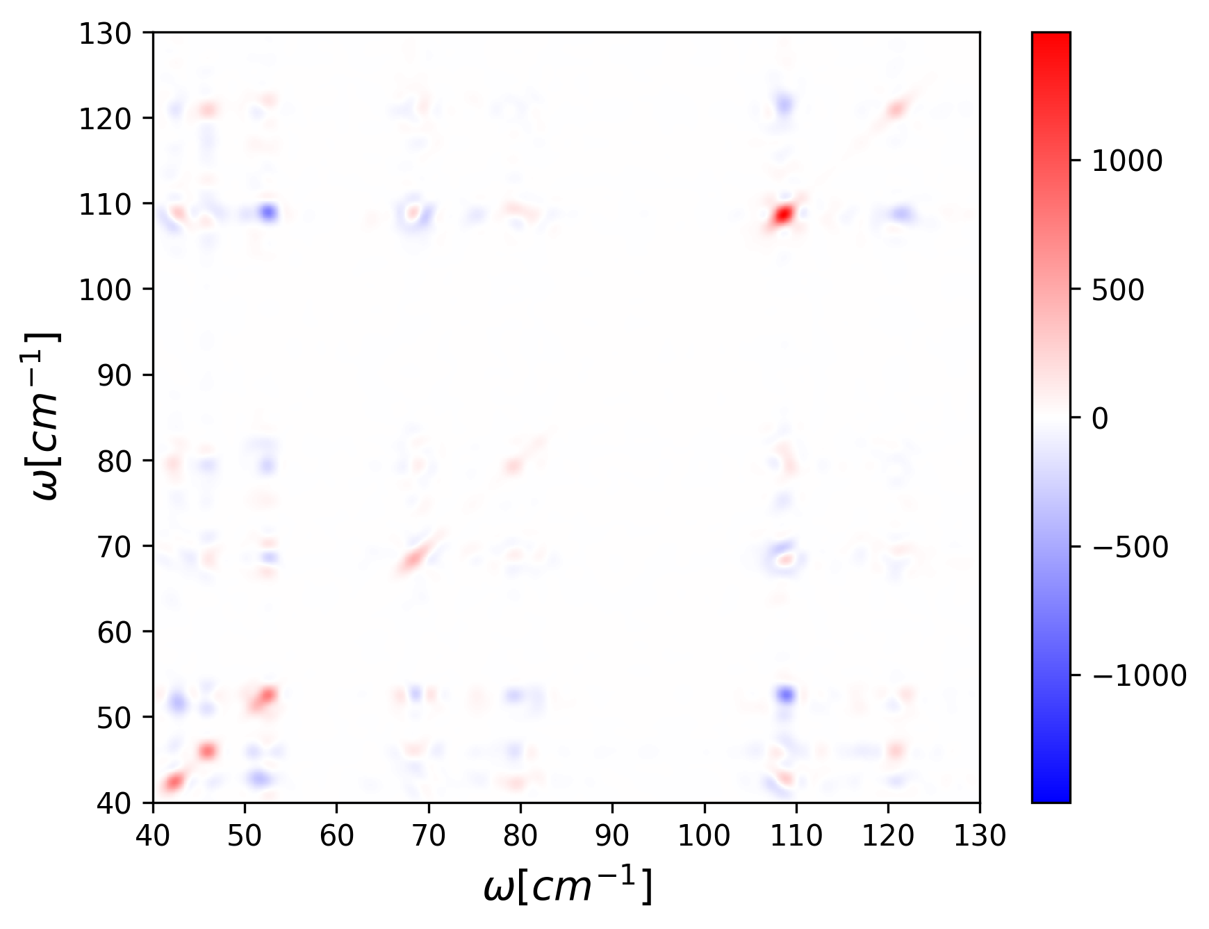
The diagonal peaks appearing in these spectra are re ferred to as autopeaks and are always positive; They represent the change in intensity at a given frequency over a given period of time. Hence, regions that change intensity a lot will have strong autopeaks, while regions that vary little will have weak autopeaks. Off-diagonal peaks, or cross-peaks, correspond to simultaneous changes (of equal or opposite signs) in intensities at two different frequencies over a given duration, indicating a possible coupling between the two corresponding vibrational modes.

'''
Function computing the dynamical VDOS spectrum, i.e. the VDOS is computed along blocks
of a given trajectory. All the block VDOS for the run are stored in spectra.'''

def blockVDOS(vel_traj, shift, block, npad):

    #The length of the block is given by shift*block_multiple.
    mlag = int(block/2)
    nblocks = int(len(vel_traj)/shift + 1 - (block/shift))

    spectra = np.zeros([nblocks, mlag+npad+1], dtype='float64')

    for (n, i) in enumerate(range(0, len(vel_traj)-block+1, shift)):

        #Construct timeseries for a given block.
        timeseries = vel_traj[i:i+block]

        #Compute the VDOS spectrum through Fourier trick.
        ft = np.fft.rfft(timeseries, axis=0)
        ac = ft*np.conjugate(ft)
        mean_ac = np.real(np.mean(ac, axis=1))
        autoCorr = np.fft.irfft(mean_ac)[:mlag+1]/np.average(timeseries**2)/block
        corrFT = dct(np.append(autoCorr*np.hanning(block)[mlag-1:], np.zeros(npad)), type=1)

        #Store the VDOS of the block.
        spectra[n] = corrFT.real

    return spectra

We can now compute all of the \(I_j(\omega)\) for a given run, and the corresponding average spectrum. In this specific example, since I am interested in the low frequency part of the spectrum, I will limit the gamma projection to the first 12 modes, excluding the acoustic ones (0,1,2).

indexes = [3,4,5,6,7,8,9,10,11]

#This dictionary will store, for every r,
#a numpy array with all the VDOS of all blocks of a given run.
spectra_run = {}

block_shift=200
block_length=4000
npad=10000

for r in runs:
    #First argument is now the velocity traj only of the NM I am interested in.
    spectra_run[r] = blockVDOS(np.take(proj[r], indexes, axis=1), block_shift, block_length, npad)

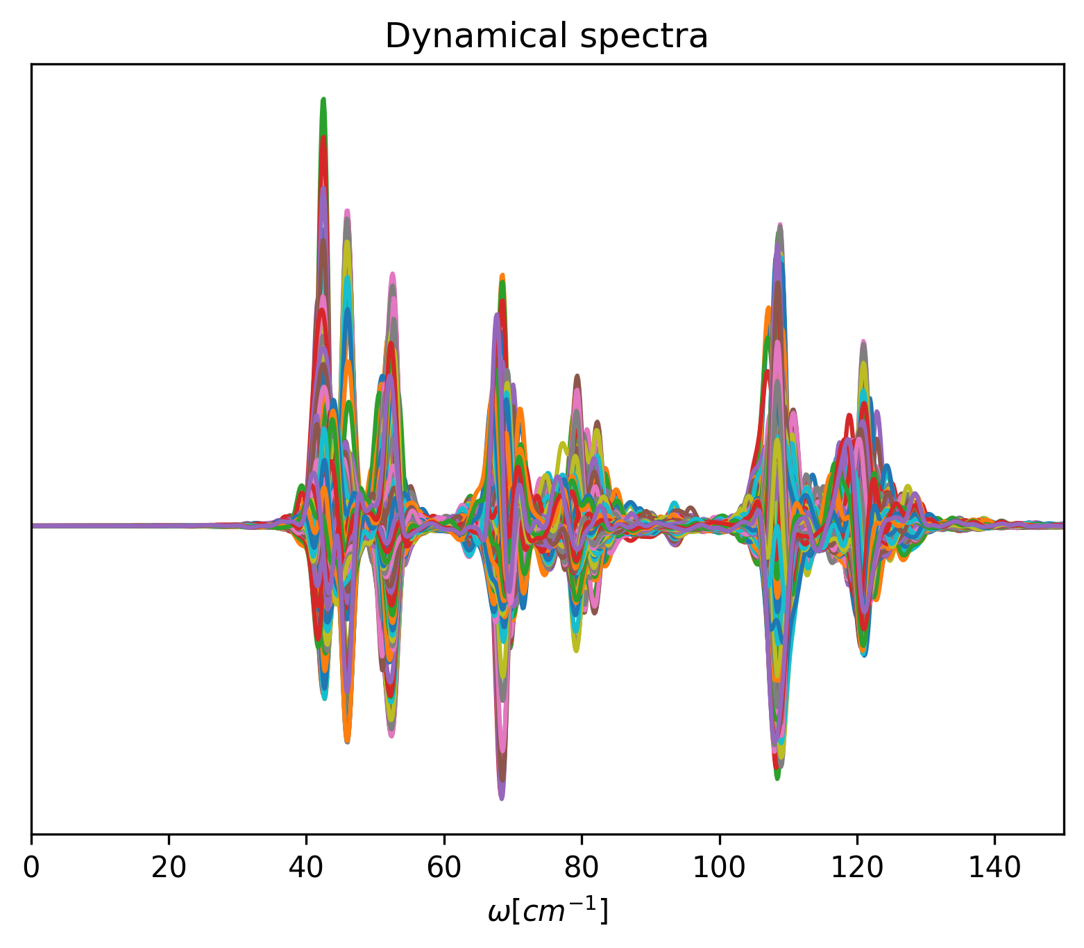
Let’s see how the collection of dynamical spectra looks like, once the average spectrum has been subtracted:

#Frequencies for the x-axis in cm-1
freq = np.fft.rfftfreq(2*int((block_length/2)+npad),timestep)*1000*33.35641 #cm-1
fig = plt.figure(dpi=300.0)

#Here I'm plotting every block VDOS of every run.
for r in runs:
    averageSpectrum = np.average(spectra_run[r],axis=0)
    for i in spectra_run[r]:
        plt.plot(freq, i-averageSpectrum)

plt.title('Dynamical spectra')
plt.xlim(0,150)
plt.yticks([])
plt.xlabel(r'$\omega [cm^{-1}]$')

Text(0.5, 0, '$\\omega [cm^{-1}]$')

2D Correlations

Here we finally compute the 2D correlations. To speed it up in case of a large dataset, a bit of jit/numba magic is used. In order to do so, we have to convert our dictionaries to numpy arrays. Let’s start from the array of dynamical spectra, subtracting the average from all the block VDOS spectra:

for r in runs:
    averageSpectrum = np.average(spectra_run[r], axis=0)
    for (i,spec) in enumerate(spectra_run[r]):
        spectra_run[r][i] = spec-averageSpectrum

spectra_list = [np.array(spectra_run[r], dtype=np.float64) for r in runs]
spectra_array = np.array([np.array(spectra_run[r], dtype=np.float64) for r in runs], dtype=np.float64)

The following functions loops on both the freq. axis in a parallel manner thanks to the numba prange function. For every couple \((\omega_j , \omega_i)\) the correlation is computed accordingly. Note that the variable freq_points sets the highest frequency we are interested at, every point is an entry in the freq array as defined previously, the spacing depends on your timestep. One can also compute the 2D correlations every N freq_points.

%%time
from numba import jit, prange

@jit(nopython=True, parallel=True)
def compute_intensity(spectra_array, freq_points, nspectra):
    intensity = np.zeros((freq_points, freq_points))

    # Loop over the frequency points
    for j in prange(freq_points):
        for k in prange(freq_points):
            # Loop over each spectrum
            for r in range(spectra_array.shape[0]):
                for i in range(spectra_array.shape[1]):  # Iterate over the second dimension
                    # Subtract the average spectrum to get dynamic spectrum (fluctuations)
                    dyn_spec = spectra_array[r, i]
                    # Compute the correlations at frequencies (j, k)
                    intensity[j, k] += dyn_spec[j] * dyn_spec[k]

    intensity /= nspectra - 1
    return intensity

# Example usage
nspectra = len(runs) * len(spectra_list[0])  # Or use the shape of the 3D array
freq_points = 1500
intensity = compute_intensity(spectra_array, freq_points, nspectra)

CPU times: user 3.41 s, sys: 145 ms, total: 3.55 s
Wall time: 1.9 s

And this is what a 2D correlation plot finally looks like:

fig = plt.figure(dpi=300.0)
ax = fig.add_subplot(111)
cax = ax.pcolormesh(freq[:1500], freq[:1500], intensity, cmap='bwr', norm=colors.CenteredNorm())
fig.colorbar(cax)

xaxis = np.arange(freq_points)

ax.set_xlim(40,130)
ax.set_ylim(40,130)
ax.set_xlabel(r'$\omega [cm^{-1}]$', fontsize = 14)
ax.set_ylabel(r'$\omega [cm^{-1}]$', fontsize = 14)

#plt.savefig('2D_100K.png')

Text(0, 0.5, '$\\omega [cm^{-1}]$')