Stochastic Thermostats

Contributed by George Trenins.

For details of the thermostats discussed here, see The Atomistic Cookbook .

Test System

We will test the effectiveness of different thermostats on a set of decoupled harmonic oscillators. For this system, thermal expectation values and time-correlation functions under the action of a (generalised) Langevin thermostat can be calculated analytically. The frequencies of our oscillators are taken from the 12-mode discretization of the exponentially damped Ohmic spectral density with a cut-off \(\omega_{\text{c}} = 500~\text{cm}^{-1}\), spanning values from \(21~\text{cm}^{-1}\) to \(1589~\text{cm}^{-1}\):

\[\omega_i = -\omega_{\text{c}} \log\left( \frac{i - 1/2}{n_{\text{bath}}} \right) \qquad i = 1,\ldots,n_{\text{bath}}.\]

We’ll be looking at a temperature of 300 K and set the masses of all the oscillators to the mass of the proton.

Langevin Themostat

There is only one parameter that can be tuned, the friction coefficient \(\gamma\) or, equivalently, its reciprocal \(\tau = 1/\gamma.\) For a harmonic oscillator with frequency \(\omega\), mass \(m\), and equilibrum centred at the origin, the position auto-correlation function at a temperature \(T\) is

\[\begin{split}\left\langle x(0) x(t)\right\rangle = \frac{ \mathrm{e}^{-t / 2 \tau} }{ \beta m \omega^2 } \times \begin{cases} \cos(\Omega t) + \frac{1}{2\Omega\tau} \sin(\Omega t) & \tau > \frac{1}{2 \omega} \\ \cosh(\Omega t) + \frac{1}{2 \Omega \tau} \sinh( \Omega t) & \tau < \frac{1}{2 \omega} \\ 1 + \frac{t}{2 \tau} & \tau = \frac{1}{2 \omega} \end{cases}\end{split}\]

where \(\Omega = \sqrt{ |\omega^2 - (1/2 \tau)^2 | } \text{ and } \beta = 1/k_{\text{B}}T\). One metric that was used to test thermostatting efficiency by Ceriotti et al. in J. Chem. Phys. 133, 124104, (2010) is the potential-energy autocorrelation function, for which we need

\[\left\langle x(0)^2 x(t)^2 \right\rangle = 2 \left\langle x(0) x(t) \right\rangle^2 + \left\langle x^2 \right\rangle^2.\]

that we can compute from Isserlis’ theorem. The fastest decorrelation time is achieved for \(\tau = 1/\omega\). When \(\tau\) is large, the system is underdamped and the decay timescale asymptotically tends to \(\tau\). At the other extreme, the decay time becomes arbitrarily long for a sufficiently small \(\tau\), so it is better to be underdamped.

Hint

When using a Langevin thermostat for a highly harmonic system, choose \(\tau\) based on the lowest relevant frequency. As a rule of thumb, \(\tau = 500~\text{fs}\) matches a lowest frequency of \(10~\text{cm}^{-1}\). Doubling the frequency halves the optimal relaxation time.

from tools import units, gle, baths
import matplotlib.pyplot as plt
import numpy as np

# Setting up the test system
u = units.atomic()
T = 300.0
beta = u.betaTemp(T)
nbath = 12
wc = u.wn2omega(500.0)      # frequency cut-off 500 cm^-1
mass = u.str2base("1 mp") # proton mass in system units
layout = (4,3)            # plotting layout
bath = baths.ExpOhmic(mass, nbath, 1.0, wc)
freqs = bath.frequencies
# Analytical results for potential/kinetic energies and their squares
x2avg = []
p2avg = []
gamma = np.min(freqs)
tau = 1/gamma
for freq in freqs:
    x2, p2 = np.diag(gle.gle_cxx([0.0], freq, gamma, beta=beta, mass=mass))
    x2avg.append(x2)
    p2avg.append(p2)
x2avg = np.asarray(x2avg)
p2avg = np.asarray(p2avg)
x4avg = 3*x2avg**2
p4avg = 3*p2avg**2

# Plotting the TCF
tmax = 2.5 # ps
npts = 1000
t_ps = np.linspace(0, tmax, npts)
t = t_ps * u.str2base("1 ps")  # in internal units
r, c = layout
fig, axarr = plt.subplots(nrows=r, ncols=c, sharex=True, sharey=True)
fig.set_size_inches([10, 10])
for i, ax in enumerate(np.ravel(axarr)):
    # Analytical time-correlation function
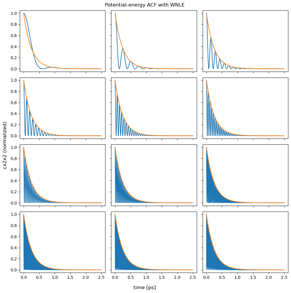
    ax.plot(t_ps,
            (2*gle.wnle_cqq(t, beta, freqs[i], tau, mass)**2) /
            (x4avg[i] - x2avg[i]**2))
    # Envelope
    ax.plot(t_ps, np.exp(-t/tau))
fig.suptitle("Potential-energy ACF with WNLE")
fig.supxlabel("time [ps]");
fig.supylabel("cx2x2 (normalized)");
fig.tight_layout()

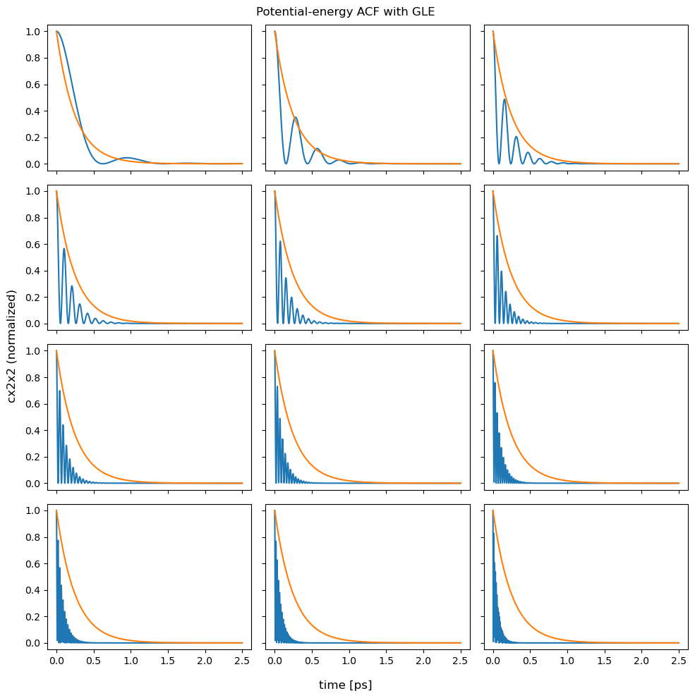
Generalized Langevin Equation thermostat (GLE)

A GLE thermostat is more flexble than white-noise Langeving (WNLE), and can enhance the sampling accuracy of the higher frequency modes without affecting too badly the sampling of slow modes. Our example uses a drift matrix from gle4md.org using a Smart sampling GLE type with the slowest sampling timescale of 2 ps, number of auxiliary DoFs = 6, and \(\omega_{\mathrm{max}} / \omega_{\mathrm{min}} = 100\).

import json

with open("thermostats/gle.json", "r") as f:
    A_pp = np.asarray(json.load(f)["A"])
fig, axarr = plt.subplots(nrows=r, ncols=c, sharex=True, sharey=True)
fig.set_size_inches([10, 10])
for i, ax in enumerate(np.ravel(axarr)):
    ref_tcf = gle.gle_cxx(t, freqs[i], A_pp, beta=beta, mass=mass)
    cxx = ref_tcf[:,0,0]
    ax.plot(t_ps, 2*cxx**2 / (x4avg[i] - x2avg[i]**2))
    ax.plot(t_ps, np.exp(-t/tau))
fig.suptitle("Potential-energy ACF with GLE")
fig.supxlabel("time [ps]");
fig.supylabel("cx2x2 (normalized)");
fig.tight_layout()

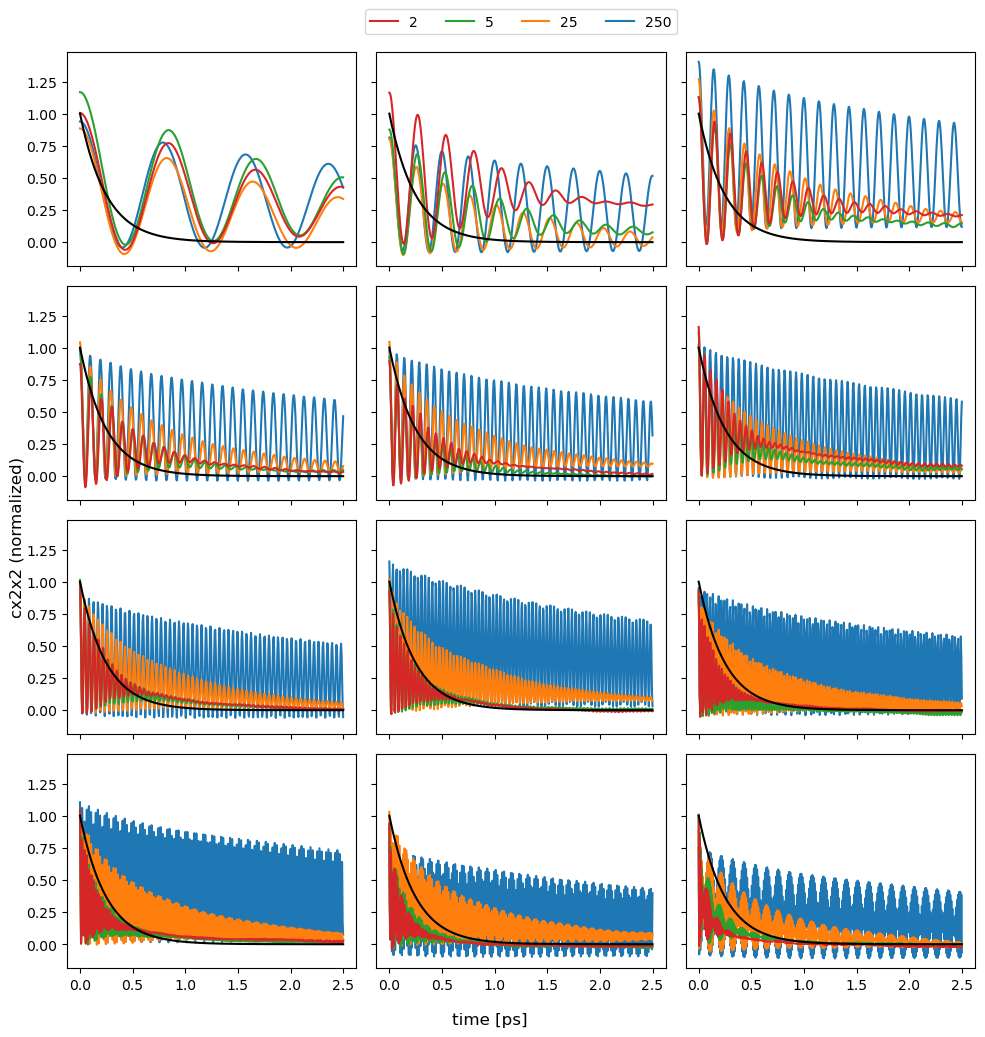
Stochastic velocity rescaling (SVR)

This, essentially, propagates the total kinetic energy according to a stochastic differential equation that preserves the Boltzmann distribution for the total kinetic energy. The thermalisation of other collective variables is not guaranteed and will be poor for our highly harmonic test case (see plot below, the legend gives the values of \(\tau\) in fs, and the black line shows the same exponential envelope as in the previous plots). For an anharmonic system, a smaller thermostat parameter \(\tau\) will generally ensure faster thermalisation.