Visualizing Molecular Orbitals
Contributed by George Trenins
This tutorial explains how to visualize molecular orbitals using FHI-aims to generate the data and OVITO to render the molecules and the isosurfaces.
Electronic structure calculation
In order to output the probability amplitude/density for the correct molecular orbitals, we must first determine their indices. For this tutorial we will consider benzene as an example. Below is the equilibrium geometry, courtesy of Hannah Bertschi, optimized using FHI-aims with the PZ LDA functional and tight defaults. Click on the title to unroll and hover in the top-right corner of the text field to access to copy button.
geometry.in
atom      -1.20547565     -0.68410539      0.00000919 C
atom      -1.19519424      0.70194528      0.00001938 C
atom      -0.01026432     -1.38603582     -0.00000186 C
atom       0.01029765      1.38606915      0.00001853 C
atom       1.19522757     -0.70191195     -0.00000272 C
atom       1.20550898      0.68413872      0.00000748 C
atom      -2.15677132     -1.22396374      0.00000987 H
atom      -2.13837649      1.25585678      0.00002809 H
atom      -0.01837692     -2.47981099     -0.00000989 H
atom       0.01841025      2.47984432      0.00002657 H
atom       2.13840983     -1.25582344     -0.00001144 H
atom       2.15680466      1.22399707      0.00000680 H
First pass
The first step is to run a single-point calculation that will allow us to determine the indices of our orbitals of interest. Remember to save the density-matrix restart files, so that you do not have to run the whole calculation from scratch on the second pass.
control.in
xc              pz-lda
spin            none
relativistic    none
charge          0.0
elsi_restart    write scf_converged

# grids and basis functions
...
Having run the calculation, examine the list of orbital energies after the final occurrence of Writing Kohn-Sham eigenvalues in the output file (the comments were added by me).
Writing Kohn-Sham eigenvalues.

State    Occupation    Eigenvalue [Ha]    Eigenvalue [eV]
    1       2.00000          -9.790481         -266.41254
  ...
   20       2.00000          -0.241127           -6.56141
   21       2.00000          -0.241127           -6.56139    # HOMO
   22       0.00000          -0.050392           -1.37123    # LUMO
   23       0.00000          -0.050392           -1.37123
  ...
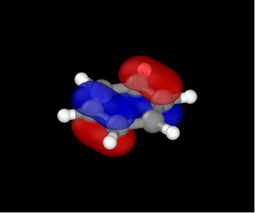
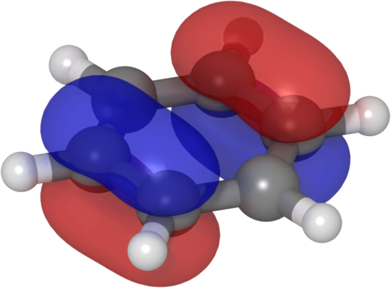
In this instance, we will be visualizing the degenerate occupied orbitals 20 and 21 (HOMO-1 and HOMO, respectively).
Second pass
Modify you control file to read
xc                 pz-lda
spin               none
relativistic       none
charge             0.0
elsi_restart       read
cube_content_unit  bohr
output             cube eigenstate 20
output             cube eigenstate 21
FHI-aims will choose sensible defaults for the three-dimensional grid on which to output the probability amplitude data. If you want to customize this, check the manual for the keywords cube origin, cube edge, and cube edge_density. If you want to output the probability density instead, change the type of the output from eigenstate to eigenstate_density.
Hint
If all you are interested in are the HOMO and/or LUMO of your system, you may specify this in your control file, e.g. output cube eigenstate homo. In this case you do not need to perform a two-pass calculation.
After running FHI-aims with the modified control file, you working directory will contain the following output files:
D_spin_01_kpt_000001.csc                # restart file from the first pass
cube_001_eigenstate_00020_spin_1.cube
cube_002_eigenstate_00021_spin_1.cube
The cube files follow an intuitive naming convention and can be visualized using VMD. However, you may achieve better results using OVITO.
Data visualization
A major advantage to OVITO is that it allows you to write visualization scripts in python. To install the python interpreter, follow the installation instructions here. I recommend using a virtual environment and including jupyter in the installation. If you are producing a one-off image or want to establish sensible visualization settings for a sequence of frames, it is convenient to perform the initial manipulations in a notebook.
Loading the data
The syntax for loading a cube file runs along the lines
from ovito.io import import_file
from ovito.pipeline import Pipeline
from ovito.data import VoxelGrid

pipeline : Pipeline = import_file(
    'cube_002_eigenstate_00021_spin_1.cube',  # name of data file
    input_format="gaussian/cube",             # optional, should be able to deduce by itself
    grid_type=VoxelGrid.GridType.PointData,   # "positioning" of data in the voxels
    generate_bonds=True                       # why not?
)
The data is loaded into a Pipeline, to which one later appends a series of post-processing operations, called Modifiers. Click here for further information on the keyword arguments.
Creating the isosurface
Calculating an isosurface is an example of an operation performed by a Modifier. You can access a complete list of all modifiers, but for our present purposes we are only interested in the aptly named CreateIsosurfaceModifier.
from typing import Optional

def append_isosurface(
        pipeline: Pipeline,
        isolevel: Optional[float] = 0.1,
        color: Optional[tuple[float,float,float]] = None,
        alpha: Optional[float] = 0.0) -> Pipeline:
    """Append a modifier to create an isosurface from volumetric data
    loaded from a FHI-aims cube file.

    Args:
        pipeline: an OVITO pipeline containing the volumetric data.
        isolevel: numerical value at which to draw the isosruface. Defaults to 0.1.
        color: isosruface color specified as an RGB tuple. Defaults to red.
        alpha: transparency of the isosurface. Defaults to 0.0.

    Returns:
        Pipeline: original pipeline with the modifier appended to it.
    """
    from ovito.vis import SurfaceMeshVis
    from ovito.modifiers import CreateIsosurfaceModifier
    # Create an object to control the visualization of the surface
    smv = SurfaceMeshVis()
    # Set the surface to be uniformly coloured
    smv.color_mapping_mode = SurfaceMeshVis.ColorMappingMode.Uniform
    if color is None:
        color = (1.0, 0.0, 0.0) # red
    # colour value as RGB tuple
    smv.surface_color = color
    # transparency level
    smv.surface_transparency = alpha
    if isolevel < 0.0:
        # invert direction of surface for negative values
        # otherwise everything from the surface *outwards* gets shaded
        smv.reverse_orientation = True
    pipeline.modifiers.append(CreateIsosurfaceModifier(
        operate_on = "voxels:imported",
        isolevel = isolevel,
        property = 'Property',
        vis = smv))
    return pipeline
You shouldn’t need to modify the arguments of CreateIsosurfaceModifier when loading FHI-aims orbital cube files. The visualization settings are controlled by the SurfaceMeshVis visualization element, which can be created first and passed as an argument to the __init__() of CreateIsosurfaceModifier, as in the example above. Alternatively, it can be modified once the modifier has already been created, to the exact same effect:
isosurface = CreateIsosurfaceModifier(
    operate_on = "voxels:imported",
    isolevel = isolevel,
    property = 'Property')
isosurface.vis.color_mapping_mode = SurfaceMeshVis.ColorMappingMode.Uniform
isosurface.vis.surface_color = color
isosurface.vis.surface_transparency = alpha
In our example, we append two modifiers, to visualize the positive and negative lobes of the HOMO:
pipeline = append_isosurface(pipeline, color=(1.0, 0.0, 0.0), isolevel=0.05, alpha=0.5)
pipeline = append_isosurface(pipeline, color=(0.0, 0.0, 1.0), isolevel=-0.05, alpha=0.5)
Modifying molecule appearance
At this stage, on further post-processing need be done on the date. All that remains are some visualization settings to modify the default appearance of the simulation cell, atoms, and bonds (if any). We may, therefore, execute the pipeline:
from ovito.data import DataCollection
data: DataCollection = pipeline.compute()
Simulation cell
The resulting DataCollection has a list of properties that describe aspects of your system, such as the simulation cell. These, properties, in turn, each have a visualization element attached to them that controls their appearance.
from ovito.data import SimulationCell
from ovito.vis import SimulationCellVis
cell: SimulationCell = data.cell
vis: SimulationCellVis = cell.vis
vis.rendering_color: tuple[float,float,float] = (0.0, 0.0, 0.0)
vis.line_width: float = 0.1     # in simulation units of length
vis.enabled: bool = False       # turn of the simulation cell completely
You can, of course, modify the visualization setting directly, as in
data.cell.vis.render_cell = False
Atoms
The appearance of the atoms is controlled via the particles property.
from ovito.data import Particles
from ovito.vis import ParticlesVis
particles: Particles = data.particles
vis: ParticlesVis = particles.vis
# scale the particle radius for all species by the same factor
vis.scaling: float = 2.0
Modifying particle colour or size by index/element is more involved and is not considered in this tutorial (refer to the documentation for more info).
Bonds
Chemical bonds are stored as a sub-object of the particles. Modifying their appearance follows the patter familiar to you by now:
from ovito.data import Bonds
from ovito.vis import BondsVis
bonds: Bonds = data.particles.bonds
vis: BondsVis = bonds.vis
# Set the width of all the bonds (in atomic units)
vis.width: float = 0.4
Making the 3D image
Now that you’ve chosen the visualization setting for the different plot elements (isosurfaces, simulation cell, atoms, and bonds), we set the scene in three-dimensional space and render it.
Positioning the camera
First, we create a Viewport, which you can think of as a window opening up onto the three-dimensional scene.
from ovito.vis import Viewport
# Insert your pipeline into the three-dimensional scene
pipeline.add_to_scene()
# Open a window on the scene
vp: Viewport = Viewport(
    type=Viewport.Type.Ortho,  # can change to Perspective
    camera_pos=3*(1,),         # position of the camera in 3D space
    camera_dir=3*(-1,),        # direction in which the camera is pointing
    fov=1.0                    # field of view of the camera
)
# Set the horizontal and vertical dimensions of the image in pixels
size: tuple[int,int] = (600, 500)
# modify camera_pos and fov to get a reasonably zoomed in view without cropping
vp.zoom_all(size=size)
It is at this stage that working in a Jupyter notebook becomes especially helpful, as you can create an interactive widget that allows you to modify the camera position:
import ipywidgets
from IPython.display import display
from ovito.gui import create_ipywidget

# width of the widget window in pixels
ww: int = 600
# keep the aspect ratio of the widget window the same as the output image
aspect: float = size[0]/size[1]
widget = create_ipywidget(vp, layout=ipywidgets.Layout(
    width=f'{ww}px', height=f'{int(ww/aspect)}px'))
display(widget)
You can rotate the molecule by left-clicking and dragging. To translate the molecule, hold down the Shift key as you left-click and drag. To zoom in and out, use the Scroll wheel. You can view the updated camera settings (e.g., for later use in a script) by executing
print(
    f"{vp.camera_dir = }\n"
    f"{vp.camera_pos = }\n"
    f"{vp.fov = }")
Rendering the image
Once you are quite satisfied with the camera angle, you can export the image by running
from ovito.vis import OpenGLRenderer
output_image_name: str = f'benzene_homo.png'
vp.render_image(
    size=size,
    alpha=True,
    crop=True,
    filename=output_image_name,
    renderer=OpenGLRenderer())
The defaults settings from the OpenGLRenderer do the job nicely, but for a highly customizable fancy alternative check out the OSPRayRenderer, which was used to produce the image below.
Tidying up
If you are processing a sequence of frames in a for-loop, you may find it helpful to remove a pipeline from the scene:
# Remove pipeline from the scene after rendering
pipeline.remove_from_scene()