A Practical Recipe for Choosing the Elevated Temperature \(T_e\) for \(T_e\)–CMD

contributed by Jorge Castro.

—

Overview

The following analysis is intended to be descriptive rather than strictly procedural. As long as your workflow remains consistent with the reasoning and methodology described below, your results should be fully reliable and comparable to those obtained in our study.

To make this process more accessible, we provide a Python script that automates all the core steps of the elevated temperature (\(T_e\)) analysis. You can either use this implementation directly or adapt it as a template to build your own analysis workflow.

Download get_Te_curve.py

—

Introduction

Trenins and Althorpe introduced the concept of a crossover radius \(r_{\text{cross}}\) — the position along a curvilinear potential below which artificial instantons may appear, leading to the curvature problem in centroid molecular dynamics (CMD).

At finite temperature, the centroid fluctuates around its equilibrium position \(r_{eq}\) according to a thermal distribution, often approximated by a Gaussian with standard deviation \(\sigma(T)\) that decreases as temperature increases.

The goal is to identify a temperature range where \(r_{\text{cross}}\) lies safely outside the tail of this distribution. In this regime, artificial instantons are avoided and CMD remains reliable. This idea is illustrated in Figure 1.

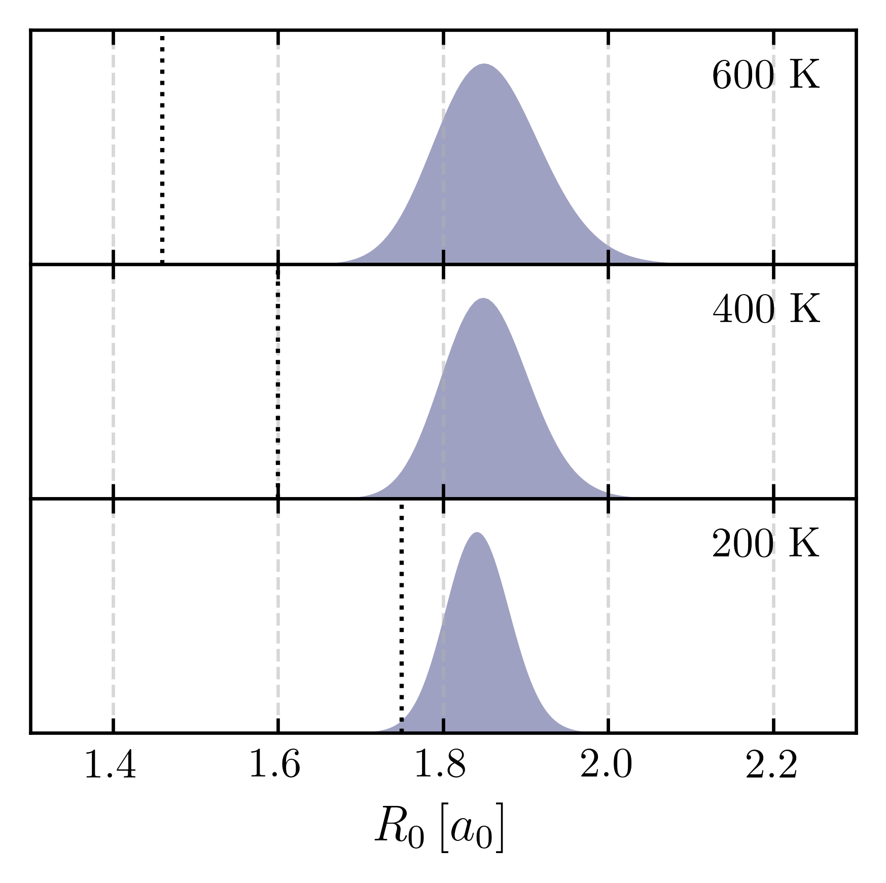
../_images/CriticalRadiusMF2.png — **Figure 1:** CMD quantum Boltzmann distributions of the centroid along the coordinate \(R_0 = \sqrt{X_0^{2} + Y_0^{2}}\) for a two-dimensional “champagne-bottle” potential representing a vibrating and rotating O–H bond. At high temperature (600 K), the centroid distribution (shaded area) remains well separated from \(r_{\text{cross}}\) (dotted line), so the curvature problem is negligible. At intermediate temperature (400 K), the tail approaches \(r_{\text{cross}}\), and at low temperature (200 K), they overlap substantially—marking the onset of artificial instantons.

The procedure outlined in our recent work provides a practical way to determine such ranges for the elevated temperature \(T_e\), using only the one-dimensional potential energy profile along the vibrational coordinate of interest.

Preparation Stage

Before determining the elevated temperature \(T_e\), ensure that a suitable potential energy surface (PES) is available for the vibrational coordinate of interest. All examples below use methylammonium lead iodide (MAPI).

1. Select Candidate Bonds

Identify bonds likely to couple with curvilinear or rotational motion — these are the most susceptible to the curvature problem.

Typical examples include O–H, N–H, C–H, or C–C stretches.

In MAPI, both N–H and C–H stretching vibrations can couple to rotational and librational modes of the molecular cation. These bonds are therefore chosen as target coordinates for generating one-dimensional potential energy scans.

2. Generate Displaced Geometries

For each selected bond:

Displace the lighter atom along the bond axis by a chosen step size (\(\pm \Delta r\)).
Generate geometries covering the specified displacement range.

The provided Python script automatically analyzes the input geometry, detects the specified bonds using a customizable interatomic distance threshold (default: 1.2 Å), and creates a dedicated directory for each identified bond.

Each directory contains an .xyz trajectory file with all displaced configurations, allowing you to visualize the motion and select representative scans for the \(T_e\) analysis.

Example command:

python get_Te_curve.py \
    --generate \
    --bonds CH NH        # Bonds of interest \
    --bond-threshold 1.2 # Angstrom \
    --geom geometry.in   # Equilibrium structure \
    --range -0.5 0.5     # Displacement range \
    --npoints 26 \
    --traj               # Generate xyz trajectories \
    --output MAPI_scans  # Output directory

3. Compute Potential Energy Scans

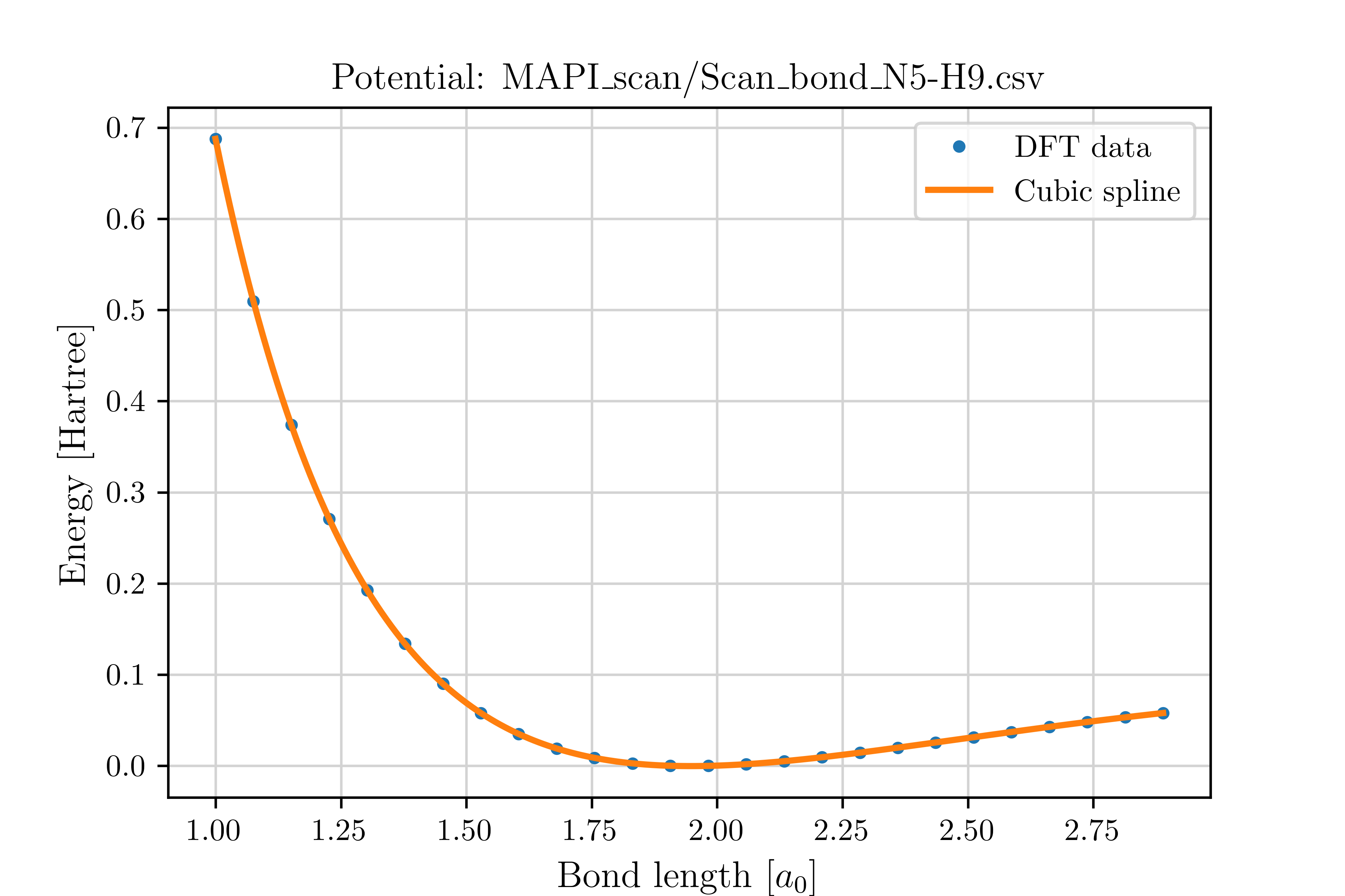
Use your preferred electronic structure method (e.g., DFT) to compute total energies for all displaced geometries. This produces the one-dimensional potential energy curves \(V(r)\) needed for the \(T_e\) analysis.

For MAPI, the selected bonds are:

N5–H9
C1–H21
C1–H26
C1–H29

Once calculations are complete, collect results and automatically generate the required .csv files using:

python get_Te_curve.py \
    --collect \
    --input Scan_bond_N5-H9  # Directory with single-point energy results \
    --prefix mapi_sp         # Prefix of the output files: mapi_sp_$Scan_Step.out \
    --range -0.5 0.5         # Angstrom \
    --npoints 26

This yields Scan_bond_N5-H9.csv.

../_images/Scan_bond_N5-H9_potential.png

\(T_e\) Calculation Overview

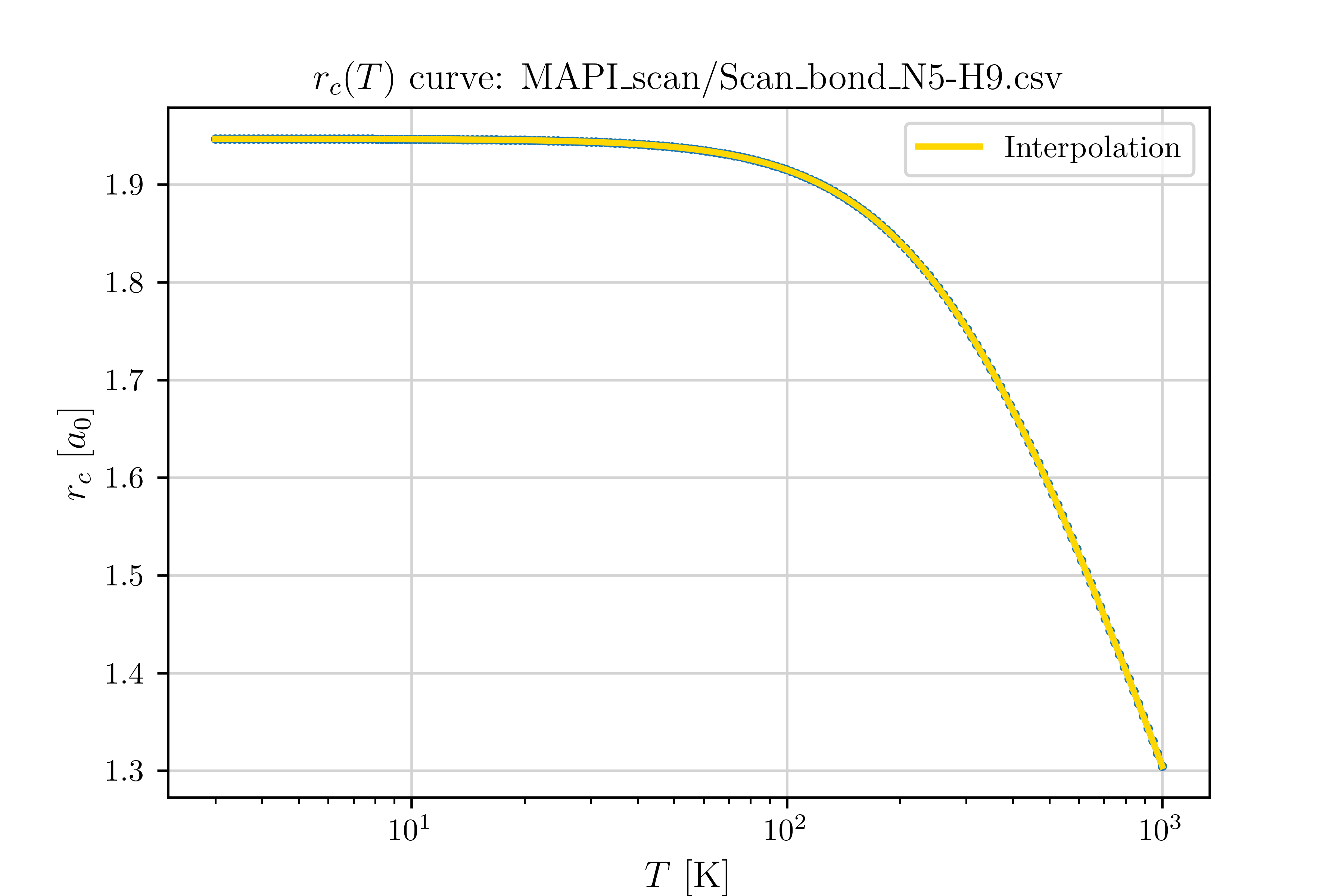
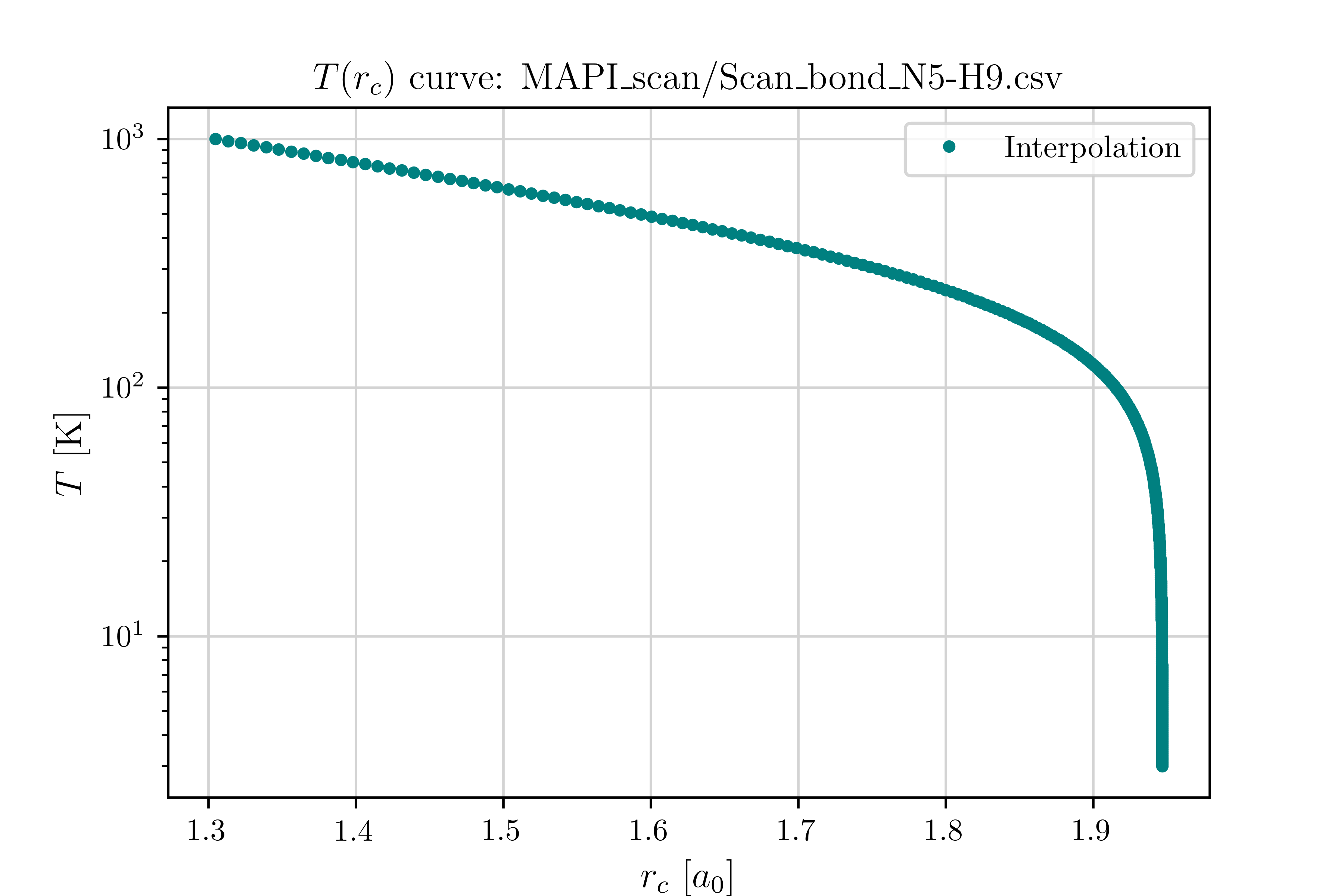
4. Determine the Crossover Radius and Mapping Functions

From the potential energy curve \(V(r)\), compute the crossover radius \(r_c(T)\) and its inverse mapping \(T(r_c)\) by solving Eq. (10) numerically.

5. Compute the Centroid Width

From the same potential, estimate the spread of centroid positions using Eq. (12). This gives the temperature-dependent width \(\sigma(T)\) of the centroid distribution.

6. Establish the Temperature Bounds

Determine the lower and upper temperature limits, \(T_{\text{low}}\) and \(T_{\text{high}}\), using Eqs. (13a) and (13b). These define the range where the curvature problem is avoided without breaking the elevated-temperature approximation.

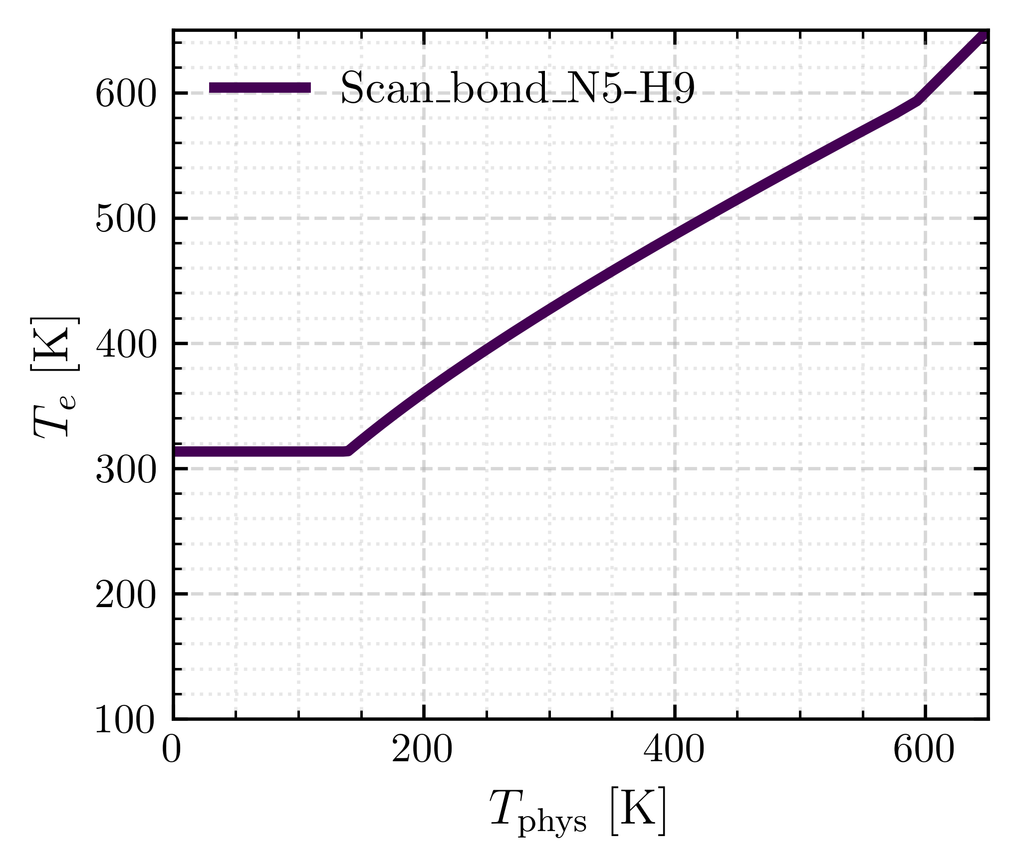
7. Construct the \(T_e(T_{\text{phys}})\) Curve

For each physical temperature \(T_{\text{phys}}\):

If \(T_{\text{phys}} < T_{\text{high}}\): Compute Eq.14 and assign: \(T_e\) as the largest of \(T_{\text{candidate}}\) and \(T_{\text{low}}\).
If \(T_{\text{phys}} > T_{\text{high}}\): set \(T_e = T_{\text{phys}}\).

This produces the final \(T_e\) vs. \(T_{\text{phys}}\) mapping.

Steps 4–7 can be executed automatically for all potential-energy scans using the command below:

python get_Te_curve.py \
    --te \
    --potentials path-to/Scan_bond_N5-H9.csv   # 1D potential files \
               path-to/Scan_bond_C1-H21.csv \
               path-to/Scan_bond_C1-H26.csv \
               path-to/Scan_bond_C1-H29.csv \
    --req-list 1.029 1.085 1.085 1.085         # Equilibrium bond lengths (Å) \
    --mred-list 1714.61 1696.49 1696.49 1696.49 # Reduced masses \
    --output results                           # Output directory \
    --tmin 3 --tmax 1000                       # Temperature range (K) \
    --tphys 110                                # Optional: target physical temperature (K) \
    --plots                                    # Optional: display intermediate plots (4–6)

The command above yields a combined plot with \(T_{e}(T_{\text{phys}})\) for all analyzed bonds.

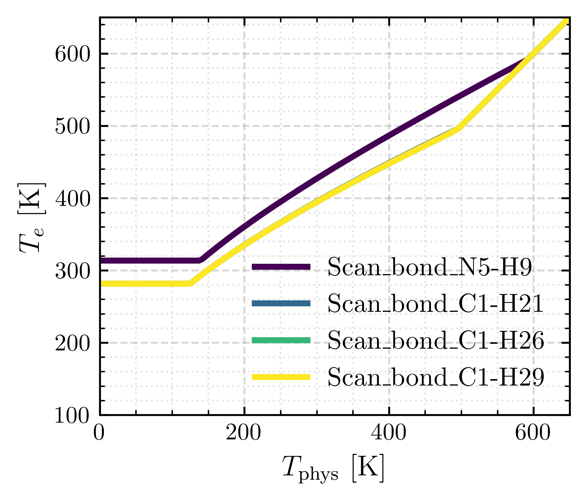
8. Select the System-Wide Elevated Temperature

If multiple bonds were analyzed, choose the highest \(T_e\) among all candidates. This ensures a single elevated temperature suitable for the entire system.