Temperature spacing for replica exchange molecular dynamics simulations
This notebooks is to generate the temperature spacing for efficeint swaping in replica exchange molecular dynamics method.
Replica Exchange Molecular Dynamics (REMD)
Enhance sampling method: overcomes the energy barriers and allows the system to sample a wider range of configurations.
NOT a TRUE Molecular dynamics simulation its just a “sampling method” because parallel tempering exchange is a unphysical move.
Sampling can be done on any intensive variables (Temperature, density, ..)
Detailed Balanced Condition:
Acceptance probability of a swap between two neighbouring temperatures
\(acc = P(T_1 \rightarrow T_2) = min(1, \exp((\beta_i -\beta_j) (U_i - U_j))\)
Questions ?
How many replicas do we need to perform REMD?
What should be the temperature spacing between the replicas?
[1]:
import os
import numpy as np
import matplotlib.pyplot as plt
from scipy.stats import linregress
[2]:
# Set global parameters
plt.rcParams['figure.figsize'] = (8, 6)  # Figure size in inches (width, height)
# plt.rcParams['figure.dpi'] = 150  # Figure resolution in dots per inch
plt.rcParams['font.family'] = 'sans-serif'  # Font family
plt.rcParams['font.sans-serif'] = 'Fira Sans'
plt.rcParams['font.size'] = 16  # Font size
plt.rcParams['axes.labelsize'] = 10  # Font size of x and y labels
plt.rcParams['axes.titlesize'] = 18  # Font size of title
plt.rcParams['axes.grid'] = True  # Show grid by default
plt.rcParams['lines.linewidth'] = 6  # Line width
plt.rcParams['lines.markersize'] = 10  # Marker size
plt.rcParams['legend.fontsize'] = 16  # Font size of legend

import logging
logging.getLogger('matplotlib.font_manager').setLevel(logging.ERROR)
[3]:
# change the working directory where you have i-pi generated short remd data
os.chdir('./short_remd_coefficient_search/')
[4]:
# one needs to sort the output from i-pi in accordance with the temperature
# !python3 remdsort.py input_remd.xml
[5]:
# Reading all the outputs of the replicas

properties = {}
for file in os.listdir():
    if file.endswith("_simulation.out") & file.startswith("SRT"):
        idx = int(file.split('_')[1])
        data = np.loadtxt(file)
        properties[idx] = data
    else :
        continue
properties = {k: v for k, v in sorted(properties.items(), key=lambda item: item[0])}
Deriving the constants for temperature spacing alorigthm
[6]:
# Constants
kb = 8.617333262145e-5 # Boltzmann constant in eV/K
Natoms = 27 # 3x3 1H-TaS2 supercell
Ndf = 3*Natoms-3 # degrees of freedom
Using last 10ps of trajectory to compute ensemble averages
[7]:
avg_potentials = np.array([np.mean(v[-10000:,6]) for k, v in properties.items()])
ensemble_temps = np.array([np.mean(v[-10000:,9]) for k, v in properties.items()])
observed_temps = np.array([np.mean(v[-10000:,3]) for k, v in properties.items()])
std_potentials = np.array([np.std(v[-10000:,6]) for k, v in properties.items()])/np.sqrt(Ndf)
[8]:
print(f'Ensemble temperatures: {ensemble_temps}\n')
print(f'Observed temperatures: {observed_temps}')
Ensemble temperatures: [ 50.  53.  56.  59.  62.  65.  68.  71.  74.  77.  80.  83.  86.  89.
  92.  95.  98. 101. 104. 107. 110.]

Observed temperatures: [ 50.26108535  53.20330219  56.25668929  59.20290569  62.27423155
  65.17519428  67.91214192  71.20242199  74.01436144  76.92244628
  79.98700373  82.81899827  85.86762277  88.79839426  91.50337063
  94.81545514  97.99874072 100.58586705 103.75503566 106.71843229
 109.8139592 ]
Computing constants:
[9]:
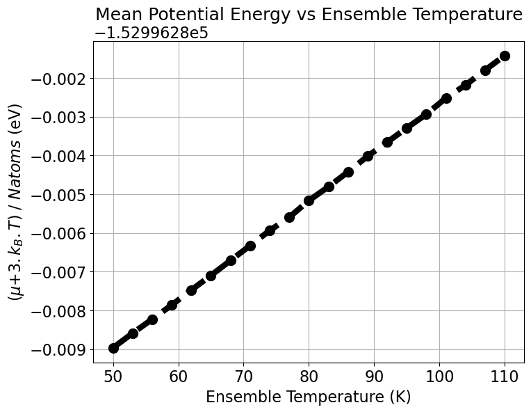
scaled_avg_potentials = (avg_potentials + 3 * kb * ensemble_temps)/Natoms
plt.figure()
plt.title('Mean Potential Energy vs Ensemble Temperature')
plt.plot(ensemble_temps, scaled_avg_potentials ,'o--', color = 'k')
plt.xlabel('Ensemble Temperature (K)')
plt.ylabel(r'($\mu$+$3.k_{B}.T$) / $Natoms$ (eV)')
slope, intercept, r_value, p_value, std_err = linregress(ensemble_temps, scaled_avg_potentials)
B0, B1 = intercept, slope
print(f'Slope B_1: {slope} eV/K, Intercept B_0: {intercept} eV, R-squared: {r_value**2}')
plt.show()
Slope B_1: 0.0001261751193934205 eV/K, Intercept B_0: -152996.29528628185 eV, R-squared: 0.9999451545563839
[10]:
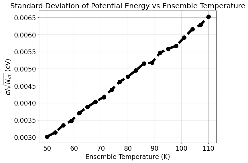
plt.figure()
plt.title('Standard Deviation of Potential Energy vs Ensemble Temperature')
plt.plot(ensemble_temps, std_potentials ,'o--', color = 'k')
plt.xlabel('Ensemble Temperature (K)')
plt.ylabel(r'$\sigma$/$\sqrt{N_{df}}$ (eV)')
slope, intercept, r_value, p_value, std_err = linregress(ensemble_temps, std_potentials)
D0, D1 = intercept, slope
print(f'Slope D_1: {slope} eV/K, Intercept D_0: {intercept} eV, R-squared: {r_value**2}')
plt.show()
Slope D_1: 5.800812914842667e-05 eV/K, Intercept D_0: 9.350154882901713e-05 eV, R-squared: 0.998153170144406
Acceptance probability
Mean and std. deviation for difference in potential energy
[11]:
import numpy as np
from scipy.special import erf
from scipy.optimize import root_scalar

class ComputeTempSpacings:
    def __init__(self, B0, B1, D0, D1, T1, Natoms, Ndf, kb):
        self.B0 = B0
        self.B1 = B1
        self.D0 = D0
        self.D1 = D1
        self.T1 = T1
        self.Natoms = Natoms
        self.Ndf = Ndf
        self.kb = kb

    def mu(self, T2):
        return self.B1 * (T2 - self.T1) * self.Natoms - 3 * self.kb * (T2 - self.T1)

    def sigma(self, T2):
        return self.D1 * np.sqrt(self.Ndf) * (T2 - self.T1)

    def C(self, T2):
        return 1/(self.kb * T2) - 1/(self.kb * self.T1)

    def prob(self, T2):
        mu_val = self.mu(T2)
        sigma_val = self.sigma(T2)
        C_val = self.C(T2)

        # for numerical stability we use log probabilities
        log_one = np.log(0.5) + np.log1p(erf(-mu_val / (np.sqrt(2) * sigma_val)))
        log_second = np.log(0.5) + C_val * mu_val + (C_val**2 * sigma_val**2) / 2
        log_third = np.log1p(erf((mu_val + C_val * sigma_val**2) / np.sqrt(2 * sigma_val**2)))

        log_prob = np.logaddexp(log_one, log_second + log_third)
        return np.exp(log_prob)

    def find_T2(self, target_prob, T2_guess_low, T2_guess_high):
        def equation(T2):
            return self.prob(T2) - target_prob

        solution = root_scalar(equation, bracket=[T2_guess_low, T2_guess_high], method='brentq')

        if solution.converged:
            return solution.root
        else:
            raise ValueError("Solution did not converge")
[13]:
Natoms = 1404 # This need to be changed for required system; here (6xroot13) 1T-TaS2 supercell
Ndf = 3*Natoms-3 # degrees of freedom
B0, B1, D0, D1 = B0, B1, D0, D1
T1, T_final = 50, 150 # initial and final temperatures
target_prob = 0.25 # target acceptance probability for swapping (T1-T2)
T2 = 0 # just a placeholder

T1s, T2s, delta_Ts = [], [], []

print(f"Total number of atoms: {Natoms}")
print(f"Degrees of freedom: {Ndf}")
print(f"Values of constants: B0={B0} eV, B1={B1} eV/K, D0={D0} eV, D1={D1} eV/K")
print(f"Inital temperature: {T1} K\tFinal temperature: {T_final} K")
print(f"Target acceptance probability for swapping (T1-T2): {target_prob}\n")
Total number of atoms: 1404
Degrees of freedom: 4209
Values of constants: B0=-152996.29528628185 eV, B1=0.0001261751193934205 eV/K, D0=9.350154882901713e-05 eV, D1=5.800812914842667e-05 eV/K
Inital temperature: 50 K        Final temperature: 150 K
Target acceptance probability for swapping (T1-T2): 0.25
[14]:
# change the directory where you want to save the temperature spacing search log

os.chdir('/classical_remd/')
print("Starting temperature spacing search...")
with open('temperature_spacing_search.log', 'w') as f:
    f.write(f"Total number of atoms: {Natoms}\n")
    f.write(f"Degrees of freedom: {Ndf}\n")
    f.write(f"Values of constants: B0={B0} eV, B1={B1} eV/K, D0={D0} eV, D1={D1} eV/K\n")
    f.write(f"Inital temperature: {T1} K\tFinal temperature: {T_final} K\n")
    f.write(f"Target acceptance probability for swapping (T1-T2): {target_prob}\n\n")

    while T2 < T_final:
        model = ComputeTempSpacings(B0, B1, D0, D1, T1, Natoms, Ndf, kb)
        try:
            T2 = model.find_T2(target_prob, T1, 1000)
            T1s.append(T1)
            T2s.append(T2)
            delta_Ts.append(T2 - T1)
            print(f"Acceptance probability: {model.prob(T2):.2f}\tT1: {T1:.2f} K\tT2: {T2:.2f} K\tDelta T: {T2 - T1:.2f} K")
            f.write(f"Acceptance probability: {model.prob(T2):.2f}\tT1: {T1:.2f} K\tT2: {T2:.2f} K\tDelta T: {T2 - T1:.2f} K\n")
        except ValueError as e:
            print(e)
        T1 = T2
Starting temperature spacing search...
Acceptance probability: 0.25    T1: 50.00 K     T2: 51.32 K     Delta T: 1.32 K
Acceptance probability: 0.25    T1: 51.32 K     T2: 52.67 K     Delta T: 1.35 K
Acceptance probability: 0.25    T1: 52.67 K     T2: 54.05 K     Delta T: 1.39 K
Acceptance probability: 0.25    T1: 54.05 K     T2: 55.48 K     Delta T: 1.42 K
Acceptance probability: 0.25    T1: 55.48 K     T2: 56.94 K     Delta T: 1.46 K
Acceptance probability: 0.25    T1: 56.94 K     T2: 58.44 K     Delta T: 1.50 K
Acceptance probability: 0.25    T1: 58.44 K     T2: 59.98 K     Delta T: 1.54 K
Acceptance probability: 0.25    T1: 59.98 K     T2: 61.56 K     Delta T: 1.58 K
Acceptance probability: 0.25    T1: 61.56 K     T2: 63.18 K     Delta T: 1.62 K
Acceptance probability: 0.25    T1: 63.18 K     T2: 64.84 K     Delta T: 1.66 K
Acceptance probability: 0.25    T1: 64.84 K     T2: 66.55 K     Delta T: 1.71 K
Acceptance probability: 0.25    T1: 66.55 K     T2: 68.30 K     Delta T: 1.75 K
Acceptance probability: 0.25    T1: 68.30 K     T2: 70.10 K     Delta T: 1.80 K
Acceptance probability: 0.25    T1: 70.10 K     T2: 71.94 K     Delta T: 1.85 K
Acceptance probability: 0.25    T1: 71.94 K     T2: 73.84 K     Delta T: 1.89 K
Acceptance probability: 0.25    T1: 73.84 K     T2: 75.78 K     Delta T: 1.94 K
Acceptance probability: 0.25    T1: 75.78 K     T2: 77.78 K     Delta T: 2.00 K
Acceptance probability: 0.25    T1: 77.78 K     T2: 79.83 K     Delta T: 2.05 K
Acceptance probability: 0.25    T1: 79.83 K     T2: 81.93 K     Delta T: 2.10 K
Acceptance probability: 0.25    T1: 81.93 K     T2: 84.09 K     Delta T: 2.16 K
Acceptance probability: 0.25    T1: 84.09 K     T2: 86.30 K     Delta T: 2.21 K
Acceptance probability: 0.25    T1: 86.30 K     T2: 88.57 K     Delta T: 2.27 K
Acceptance probability: 0.25    T1: 88.57 K     T2: 90.90 K     Delta T: 2.33 K
Acceptance probability: 0.25    T1: 90.90 K     T2: 93.30 K     Delta T: 2.39 K
Acceptance probability: 0.25    T1: 93.30 K     T2: 95.75 K     Delta T: 2.46 K
Acceptance probability: 0.25    T1: 95.75 K     T2: 98.28 K     Delta T: 2.52 K
Acceptance probability: 0.25    T1: 98.28 K     T2: 100.86 K    Delta T: 2.59 K
Acceptance probability: 0.25    T1: 100.86 K    T2: 103.52 K    Delta T: 2.66 K
Acceptance probability: 0.25    T1: 103.52 K    T2: 106.25 K    Delta T: 2.73 K
Acceptance probability: 0.25    T1: 106.25 K    T2: 109.04 K    Delta T: 2.80 K
Acceptance probability: 0.25    T1: 109.04 K    T2: 111.91 K    Delta T: 2.87 K
Acceptance probability: 0.25    T1: 111.91 K    T2: 114.86 K    Delta T: 2.95 K
Acceptance probability: 0.25    T1: 114.86 K    T2: 117.89 K    Delta T: 3.02 K
Acceptance probability: 0.25    T1: 117.89 K    T2: 120.99 K    Delta T: 3.10 K
Acceptance probability: 0.25    T1: 120.99 K    T2: 124.18 K    Delta T: 3.19 K
Acceptance probability: 0.25    T1: 124.18 K    T2: 127.45 K    Delta T: 3.27 K
Acceptance probability: 0.25    T1: 127.45 K    T2: 130.80 K    Delta T: 3.36 K
Acceptance probability: 0.25    T1: 130.80 K    T2: 134.25 K    Delta T: 3.44 K
Acceptance probability: 0.25    T1: 134.25 K    T2: 137.78 K    Delta T: 3.53 K
Acceptance probability: 0.25    T1: 137.78 K    T2: 141.41 K    Delta T: 3.63 K
Acceptance probability: 0.25    T1: 141.41 K    T2: 145.13 K    Delta T: 3.72 K
Acceptance probability: 0.25    T1: 145.13 K    T2: 148.95 K    Delta T: 3.82 K
Acceptance probability: 0.25    T1: 148.95 K    T2: 152.87 K    Delta T: 3.92 K
/tmp/ipykernel_15522/1430485309.py:31: RuntimeWarning: invalid value encountered in double_scalars
  log_one = np.log(0.5) + np.log1p(erf(-mu_val / (np.sqrt(2) * sigma_val)))
/tmp/ipykernel_15522/1430485309.py:33: RuntimeWarning: invalid value encountered in double_scalars
  log_third = np.log1p(erf((mu_val + C_val * sigma_val**2) / np.sqrt(2 * sigma_val**2)))
/tmp/ipykernel_15522/1430485309.py:35: RuntimeWarning: invalid value encountered in logaddexp
  log_prob = np.logaddexp(log_one, log_second + log_third)
/tmp/ipykernel_15522/1430485309.py:31: RuntimeWarning: divide by zero encountered in log1p
  log_one = np.log(0.5) + np.log1p(erf(-mu_val / (np.sqrt(2) * sigma_val)))
/tmp/ipykernel_15522/1430485309.py:33: RuntimeWarning: divide by zero encountered in log1p
  log_third = np.log1p(erf((mu_val + C_val * sigma_val**2) / np.sqrt(2 * sigma_val**2)))
[15]:
print(np.asarray(T2s).shape)
(43,)