Phonopy in Python
Maintainer: Zekun Lou, Shubham Sharma
This notebook provides a straightforward guide to using phonopy in Python scripts with graphite as example.
It serves as a starting point for those who want to avoid the black box of phonopy shell commands, and prefer to integrate phonopy into their own Python scripts for customizing workflows.
NOTE: To perform a phonon calculation, one needs an relaxed structure. Please relax the structure using your preferred methods (DFT or MLIPs) before computing phonons.
We have done all DFT calculations in this tutorial.
Although this document is fairly detailed, the core Python code is concise (no more than some imports and simple function calls). The additional content is included to enhance clarity and provide better explanations. You can copy and modify the code snippets to fit your specific needs.
The workflow is as follows:
Converge the k-grid for the primitive cell and relax the primitive cell by
FHI-aims.Generate supercells with displacements using
phonopy.Perform force calculations for each supercell using DFT softwares or machine learning interatomic potentials (MLIPs).
Here example for
FHI-aimsandMACEare provided.
Extract forces and construct force constants by
phonopy.This serves as a milestone for post-processing.
Compute the phonon band structure using
phonopy.
The project’s file structure is as follows:
${PROJECT_ROOT}
├── fd_runs
│   ├── sc_5  # for example, supercell size 5x5x5
│   │   ├── aims_runs
│   │   │   └── {0..${n}}  # directories for each run
│   │   ├── geoms_disp
│   │   │   └── {0..${n}}.xyz
│   │   ├── logs
│   │   ├── control.force.in  # for FHI-aims force calculation
│   │   ├── force_constants.h5  # force_constants hdf5 file saved by phonopy
│   │   ├── phono_bandstr.meV.png  # phonon band structure plot
│   │   └── phonopy_params.yaml  # phonopy meta-settings for this calculation
│   └── sc_${sc}  # other supercell sizes
├── relax_cell  # dir for cell relaxation calculations
│   └── relaxed.xyz  # the relaxed cell
└── phonopy_in_python.ipynb  # this file
[1]:
""" change dir to ensure the file relative paths, you shall change it for your own project """
import os

PROJECT_ROOT = os.getcwd()
if PROJECT_ROOT.endswith("docs/source"):
    PROJECT_ROOT = os.path.join(PROJECT_ROOT, "phonopy_simple")
elif PROJECT_ROOT.endswith("phonopy_simple"):
    pass
print(PROJECT_ROOT)
/home/zekunlou/Projects/pj_docs/docs_howtos/docs/source/phonopy_simple
[ ]:
import matplotlib.pyplot as plt
import numpy
from ase.atoms import Atoms as aseAtoms
from ase.io import read, write
from ase.build import make_supercell

import h5py  # for compact binary force constants storage
from phonopy import Phonopy  # main class
from phonopy.cui.load import load as load_phonopy  # load from input yaml files
from phonopy.file_IO import read_force_constants_hdf5, write_force_constants_to_hdf5  # read/write FCs
from phonopy.phonon.band_structure import get_band_qpoints_and_path_connections  # band structure q-points
from phonopy.structure.atoms import PhonopyAtoms  # phonopy atoms class
[ ]:
""" prepare useful functions for structure class conversion """

def atoms_ase2ph(atoms: aseAtoms):
    if not numpy.all(atoms.get_pbc()):
        print("WARNING: for PhonopyAtoms the pbc must be T T T. Set to T T T.")
    return PhonopyAtoms(
        symbols=atoms.get_chemical_symbols(),
        cell=atoms.get_cell().array,
        positions=atoms.get_positions(),
    )

def atoms_ph2ase(atoms: PhonopyAtoms):
    return aseAtoms(
        symbols=atoms.symbols,
        cell=atoms.cell,
        positions=atoms.positions,
        pbc=True,
    )
Generate displaced structures
[4]:
""" prepare parameters """

supercell = 5
work_dpath = f"{PROJECT_ROOT}/fd_runs/sc_{supercell}"
displacement = 1e-2
xyz_eq_fpath = f"{PROJECT_ROOT}/relax_cell/relaxed.xyz"

""" prepare directories and files """

geoms_dpath = f"{work_dpath}/geoms_disp"
aims_dpath = f"{work_dpath}/aims_runs"
logs_dpath = f"{work_dpath}/logs"
phonpy_params_fpath = f"{work_dpath}/phonopy_params.yaml"
force_constants_fpath = f"{work_dpath}/force_constants.h5"
band_structure_fpath = f"{work_dpath}/band_structure.h5"
[os.makedirs(dpath, exist_ok=True) for dpath in (geoms_dpath, aims_dpath, logs_dpath)]
atoms_prim = read(xyz_eq_fpath)

""" better load from phonopy_params.yaml for reproducibility """

if os.path.exists(phonpy_params_fpath):
    phonon = load_phonopy(phonpy_params_fpath)
    print(f"Loaded phonopy parameters from {phonpy_params_fpath}")
else:
    phonon = Phonopy(
        unitcell=atoms_ase2ph(atoms_prim),
        supercell_matrix=numpy.eye(3, dtype=int) * supercell,
    )
    phonon.generate_displacements(distance=displacement)
    phonon.save(phonpy_params_fpath)

""" write the displaced supercells for FHI-aims calculation """
""" for MLIPs: you can directly produce the force_sets with shape (n_supercells, n_atoms, 3), as the next cell """
for i, this_sc in enumerate(phonon.supercells_with_displacements):
    write(f"{geoms_dpath}/{i}.xyz", atoms_ph2ase(this_sc))
    os.makedirs(f"{aims_dpath}/{i}", exist_ok=True)
    write(f"{aims_dpath}/{i}/geometry.in", atoms_ph2ase(this_sc), format="aims")
Loaded phonopy parameters from /home/zekunlou/Projects/pj_docs/docs_howtos/docs/source/phonopy_simple/fd_runs/sc_5/phonopy_params.yaml
Here we have generated the displaced structures (with symmetry considerations) to get the force constants. We need to perform single point calculations using FHI-aims or MLIPs, and then translate them to force constants using phonopy.
Calculate forces and then compute force constants
With generated structures in ${PROJECT_ROOT}/fd_runs/sc_${supercell}/geoms_disp/, one shall perform force calculations using FHI-aims.
Pre-calculation is done with results in ${PROJECT_ROOT}/fd_runs/sc_${supercell}/aims_runs/{0..n}/.
[5]:
""" FHI-aims: load force constants and save it h5, because it could be slow, especially for large supercells and repeated calculations """

if os.path.exists(force_constants_fpath):
    phonon.force_constants = read_force_constants_hdf5(force_constants_fpath)
    print(f"Loaded force constants from {force_constants_fpath}")
else:
    """Load from aims output. Please rewrite this part for your own code."""
    force_sets = numpy.array([
        read(os.path.join(f"{aims_dpath}/{task_idx}/aims.out"), format="aims-output").get_forces()
        for task_idx in sorted(os.listdir(aims_dpath), key=lambda x: int(x))
    ])
    phonon.produce_force_constants(
        forces=force_sets,
        calculate_full_force_constants=False,
    )  # we are generating compact force constants here
    write_force_constants_to_hdf5(
        phonon.get_force_constants(),
        filename=force_constants_fpath,
    )
print(f"{phonon.force_constants.shape=}")
Loaded force constants from /home/zekunlou/Projects/pj_docs/docs_howtos/docs/source/phonopy_simple/fd_runs/sc_5/force_constants.h5
phonon.force_constants.shape=(4, 500, 3, 3)
MLIPs can also serve as a calculator here, and ASE calculator interface makes it handy.
Please check this python script for running phonopy with MACE calculator.
Plot and save phonon band structure
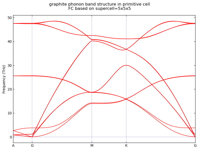
With computed force constants, we can calculate, plot, and save the phonon bands and modes.
Website https://henriquemiranda.github.io/phononwebsite/phonon.html is very useful for interactive visualization of phonon bands with the data we have generated so far. It is highly recommended to give it a try.
[9]:
""" calculate phonon band structure """

special_points = {  # for hexagon cell with gamma = 60.0 deg
    "G": [0.0, 0.0, 0.0],
    "M": [1 / 2, 1 / 2, 0.0],
    "K": [1 / 3, 2 / 3, 0.0],
    "A": [0.0, 0.0, 1 / 2],
}

bz_labels = ["A", "G", "M", "K", "G"]
kpath = [[special_points[label] for label in bz_labels]]  # must be 2-level list
kpts, connections = get_band_qpoints_and_path_connections(kpath, npoints=101)

phonon.run_band_structure(kpts, path_connections=connections, labels=bz_labels)
# phonon.write_hdf5_band_structure(filename=band_structure_fpath)  # if you want to save detailed band structure data

fig, ax = plt.subplots(1, 1, figsize=(8, 6))
phonon._band_structure.plot([ax])  # a hack here, should be List[Axes]
xscale_factor = (
    max([numpy.max(fq) for fq in phonon._band_structure.frequencies])
    / phonon._band_structure.distances[-1][-1]
    * 1.5
)  # this can be found in phonopy src code
for d in phonon._band_structure.distances:
    ax.axvline(d[-1] * xscale_factor, color="b", linestyle=":", linewidth=0.5)

ax_unit = ["meV", "cm-1", "THz"][2]  # choose your preferred unit
if ax_unit == "meV":
    ax.set_ylabel("Energy (meV)")
    ax.set_ylim(ax.get_ylim())
    ax_yticks_in_meV = numpy.arange(0, 220, 20)
    ax.set_yticks(ax_yticks_in_meV / 4.1357, ax_yticks_in_meV)
elif ax_unit == "cm-1":
    ax_yticks_in_cm = numpy.arange(0, 1800, 200)
    ax.set_yticks(ax_yticks_in_cm / 4.1357 / 8.1, ax_yticks_in_cm)
    ax.set_ylabel("Frequency (cm$^{-1}$)")
elif ax_unit == "THz":
    ax.set_ylabel("Frequency (THz)")
else:
    raise ValueError(f"Unknown ax_unit: {ax_unit}")

fig.suptitle(
    f"graphite phonon band structure in primitive cell\nFC based on supercell={supercell}x{supercell}x{supercell}"
)
fig.tight_layout()
fig = plt.gcf()
fig.savefig(f"{work_dpath}/phonon_bandstr.{ax_unit}.png", dpi=300, transparent=True)
[9]:
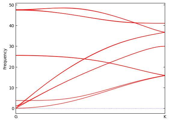
"""save for visualization"""
bz_labels = ["G", "K",]
kpath = [[special_points[label] for label in bz_labels]]  # must be 2-level list
kpts, connections = get_band_qpoints_and_path_connections(kpath, npoints=101)

phonon.run_band_structure(kpts, path_connections=connections, labels=bz_labels, with_eigenvectors=True,)
phonon.write_hdf5_band_structure(filename=f"{work_dpath}/band_structure.GK.h5")
phonon._band_structure.plot([plt.gca()])
Phonopy using command line for FHI-aims
Phonopy calculation parameter:
phonopy -d --dim="5 5 5" --tolerance=1e-4 --aims
Then one creates FHI-aims calculation folders for each structure:
for i in {001..008}; do cd disp-${i}; cp ../control.in ./; cp ../geometry.in.$i ./; cd ../; done
and then perform DFT calculations. Once finished, use the following line to create force constants:
phonopy -f disp-???/aims.out # Create FORCESET file
Then create a mesh.conf file copy below parameters, k-path A-\(\Gamma\)-M-K-\(\Gamma\):
DIM = 5 5 5
BAND = 0.0 0.0 0.5  0.0 0.0 0.0  0.5 0.5 0.0  0.333 0.667 0.0  0.0 0.0 0.0
BAND_POINTS = 101
EIGENVECTORS = .TRUE.
HDF5 = .TRUE.
BAND_CONNECTION = .TRUE.
Finally, compute phonon band structure and save plot:
phonopy -s mesh.conf --tolerance=1e-4 >> phonopy.out
For saving plot also use -p flag before -s.
Phonon mode visualization
[10]:
"""
in phonopy.harmonics.dynamical_matrix.DynamicalMatrix._run_py_dynamical_matrix,
the phase factor is phase.append(np.vdot(vec, q) * 2j * np.pi)  # positive sign
"""

def generate_phonon_visuals(
    atoms: aseAtoms,
    ph_eigvec: numpy.ndarray,
    k: numpy.ndarray,
    supercell: numpy.ndarray,
    num_frames: int = 16,
    amp_factor: float = 1.0,  # mass-scaling factor
    comment: str = "",
) -> list:
    """
    Generate phonon frames for visualization.
    For postprocessing phonopy output for visualization.

    Note:
        The phonon eigenvectors should be like phonopy, i.e. bloch phase applied to each atom but not unit cell.

    Args:
        atoms (ase.atoms.Atoms): The atomic structure.
        ph_eigvec (numpy.ndarray): Phonon eigenvector, better from phonopy.
        k (numpy.ndarray): Wave vector contains the 2*pi factor.
        supercell (numpy.ndarray): Supercell transformation matrix.
        num_frames (int, optional): Number of frames to generate. Defaults to 16.
        amp_factor (float, optional): Amplitude scaling factor. Defaults to 1.0.
        comment (str, optional): Comment to add to each frame. Defaults to "".

    Returns:
        list: List of Atoms objects representing the frames.

    Reference:
        Eq.27 in A. Togo, L. Chaput, T. Tadano, and I. Tanaka, Implementation strategies in phonopy and phono3py,
        J. Phys.: Condens. Matter 35, 353001 (2023).
    """
    assert ph_eigvec.ndim == 1, f"ph_eigvec should be a 1D array, but got {ph_eigvec.ndim}D"
    assert ph_eigvec.size == len(atoms) * 3, \
        f"ph_eigvec size should be (natoms * 3)=({len(atoms) * 3}), but got {ph_eigvec.size}"
    assert supercell.ndim == 2 and supercell.shape[0] == supercell.shape[1] == 3, \
        f"supercell should be a 3x3 matrix, but got shape {supercell.shape}"

    # Generate the supercell
    supercell_atoms = make_supercell(atoms, supercell)
    sc_positions = supercell_atoms.get_positions()

    # Repeat phonon eigenvector for the supercell
    natoms = len(atoms)
    sc_eigvec = numpy.tile(ph_eigvec.reshape(natoms, 3), (len(supercell_atoms) // natoms, 1))  # shape (n_sc_atoms, xyz)

    # Apply Bloch phase correction for each atom in the supercell
    bloch_phase_factor = numpy.exp(1j * (sc_positions @ k))[:, None]  # shape (n_sc_atoms, 1)

    # Apply Bloch phase to eigenvector
    sc_eigvec = (sc_eigvec * bloch_phase_factor)

    # Compute phonon displacements
    ph_phase = numpy.angle(sc_eigvec)  # shape (n_sc_atoms, xyz)
    ph_amp = amp_factor * numpy.abs(sc_eigvec) * (supercell_atoms.get_masses()**(-0.5))[:, None]  # shape (n_sc_atoms, xyz)
    ph_disp_time = numpy.linspace(0, 2 * numpy.pi, num_frames)  # omega*t for one period

    # Calculate displacements for each frame
    ph_disp = ph_amp[None, :] * numpy.sin(
        ph_phase[None, :] + ph_disp_time[:, None, None]
    )  # shape (n_frames, n_sc_atoms, xyz)

    # Generate frames
    ph_frames = []
    for i in range(num_frames):
        this_atoms = supercell_atoms.copy()
        this_atoms.positions = sc_positions + ph_disp[i]
        this_atoms.info["comment"] = comment
        ph_frames.append(this_atoms)

    return ph_frames
[ ]:
work_dpath = f"{PROJECT_ROOT}/fd_runs/sc_5"
atoms = read(f"{PROJECT_ROOT}/relax_cell/relaxed.xyz")

with h5py.File(f"{work_dpath}/band_structure.GK.h5", "r") as h5:
    # show the keys and arrays in the h5 file
    print(h5.keys())
    for k in h5.keys():
        if h5[k].size < 10:
            print(f"{k=}, shape={h5[k].shape}, content={h5[k][()]}")
        else:
            print(f"{k=}, shape={h5[k].shape}")
        if k == "frequency":
            data = h5[k][()]
    ph_kpath_frac = h5["path"][0,:]
    ph_freqs = h5["frequency"][0,:]
    ph_eigvecs = h5["eigenvector"][0,:]  # shape (n_kpoints, n_atoms*3, n_bands/n_modes)
ph_kpath = ph_kpath_frac @ atoms.cell.reciprocal()  # without the 2pi factor
print(f"{ph_freqs.shape=}, {ph_eigvecs.shape=}, {ph_kpath.shape=}")

# Example usage
os.makedirs(ph_viz_dpath:=f"{PROJECT_ROOT}/fd_runs/sc_5/ph_GK_viz_sc", exist_ok=True)
supercell_matrix = numpy.array([[10, 0, 0], [0, 10, 0], [0, 0, 1]])  # Example 10x10x1 supercell

kpt_idx, band_idx = 10, 2
for band_idx in (2, 3):  # TA and TA(antisymm) mode
    ph_eigvec = ph_eigvecs[kpt_idx][:, band_idx]
    ph_frames = generate_phonon_visuals(
        atoms,
        ph_eigvec,
        k=2 * numpy.pi * ph_kpath[kpt_idx],  # Convert k-point to reciprocal space
        supercell=supercell_matrix,
        comment=f"seg=GK,kpt_idx={kpt_idx},band_idx={band_idx}"
    )
    write(f"{ph_viz_dpath}/GK_kpt_{kpt_idx}_band_{band_idx}.xyz", ph_frames)
<KeysViewHDF5 ['distance', 'eigenvector', 'frequency', 'label', 'nqpoint', 'path', 'segment_nqpoint']>
k='distance', shape=(1, 101)
k='eigenvector', shape=(1, 101, 12, 12)
k='frequency', shape=(1, 101, 12)
k='label', shape=(1, 2), content=[[b'G' b'K']]
k='nqpoint', shape=(1,), content=[101]
k='path', shape=(1, 101, 3)
k='segment_nqpoint', shape=(1,), content=[101]
ph_eigvals.shape=(101, 12), ph_eigvecs.shape=(101, 12, 12), ph_kpath.shape=(101, 3)
Rendering phonon modes with OVITO
Then you can put the frames into OVITO (docs on rendering) or VMD for visualization. After rendering by OVITO and concatenating by ffmpeg, we get
For TA (transverse acoustic) mode:
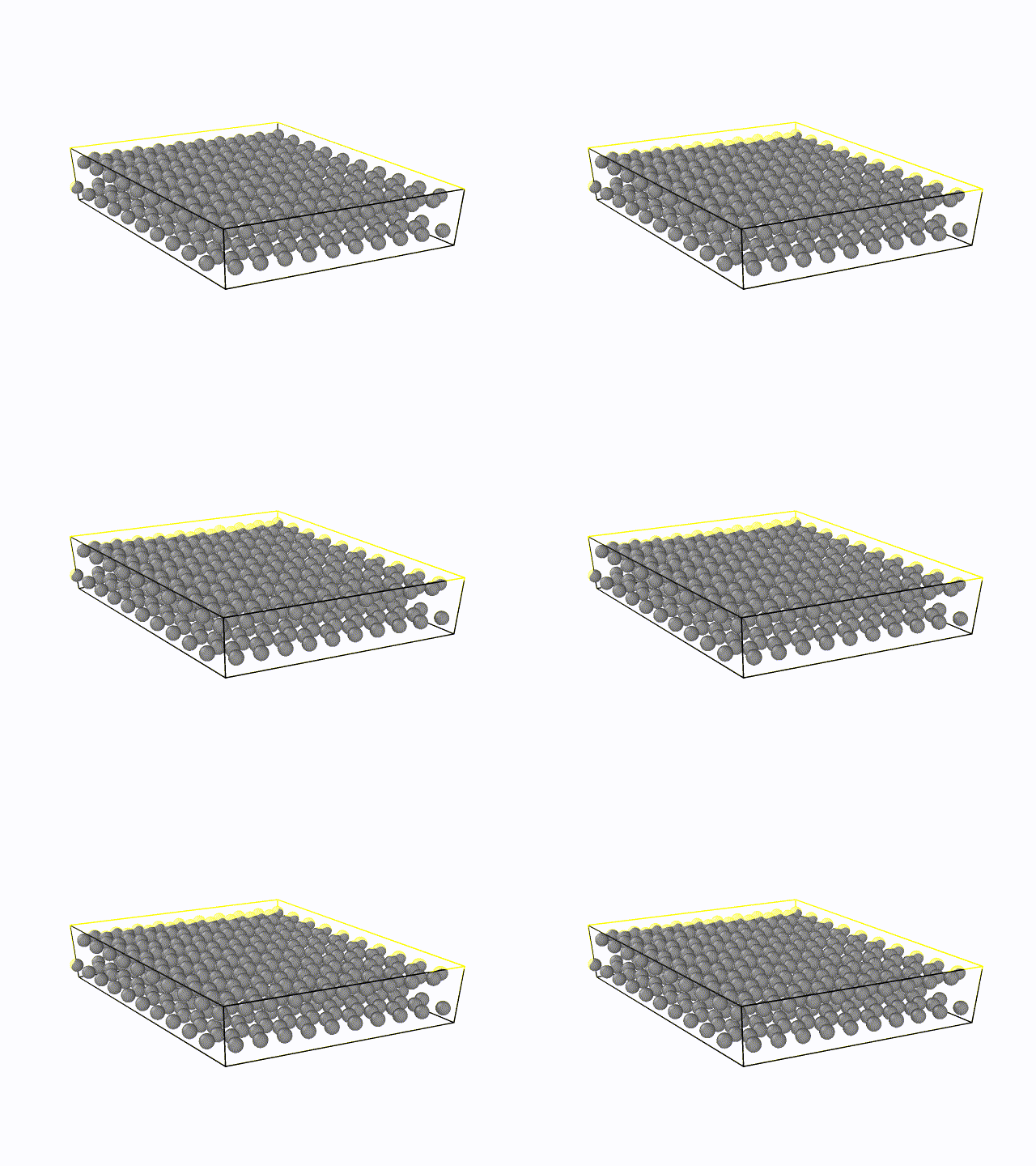
For T \(\!\!\tilde{A}\) (transverse acoustic anti-symmetric) mode:
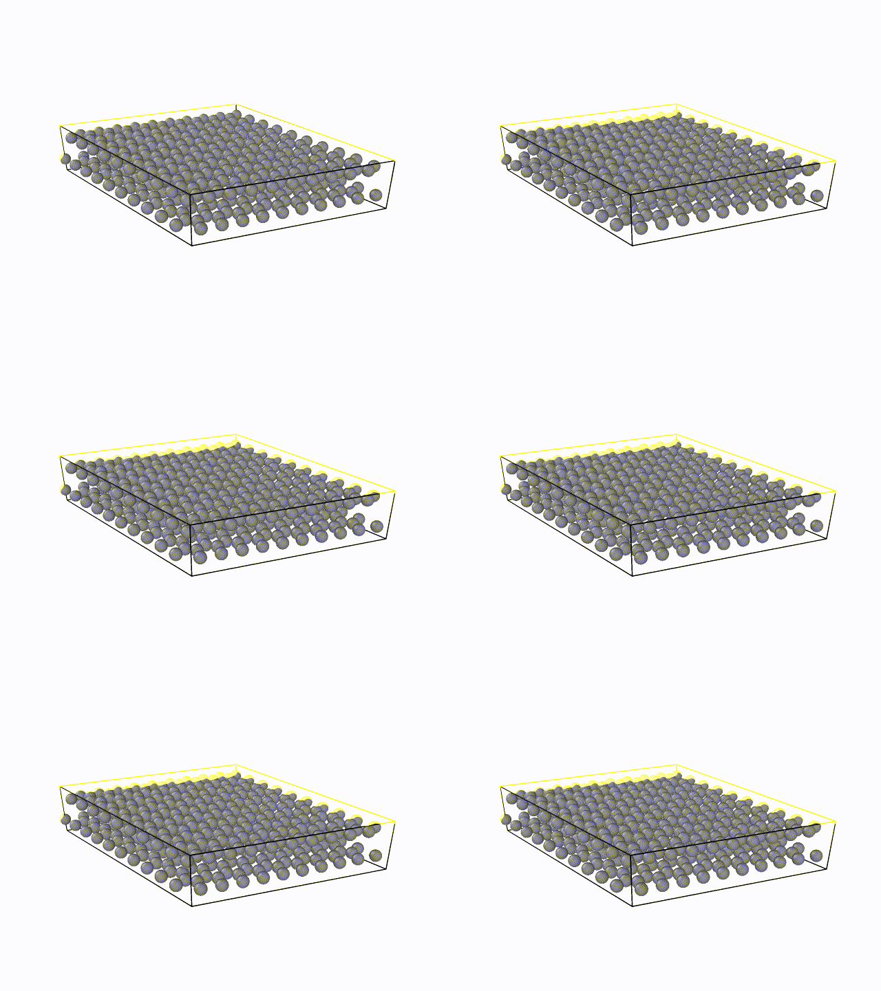
Or OVITO python script for rendering.
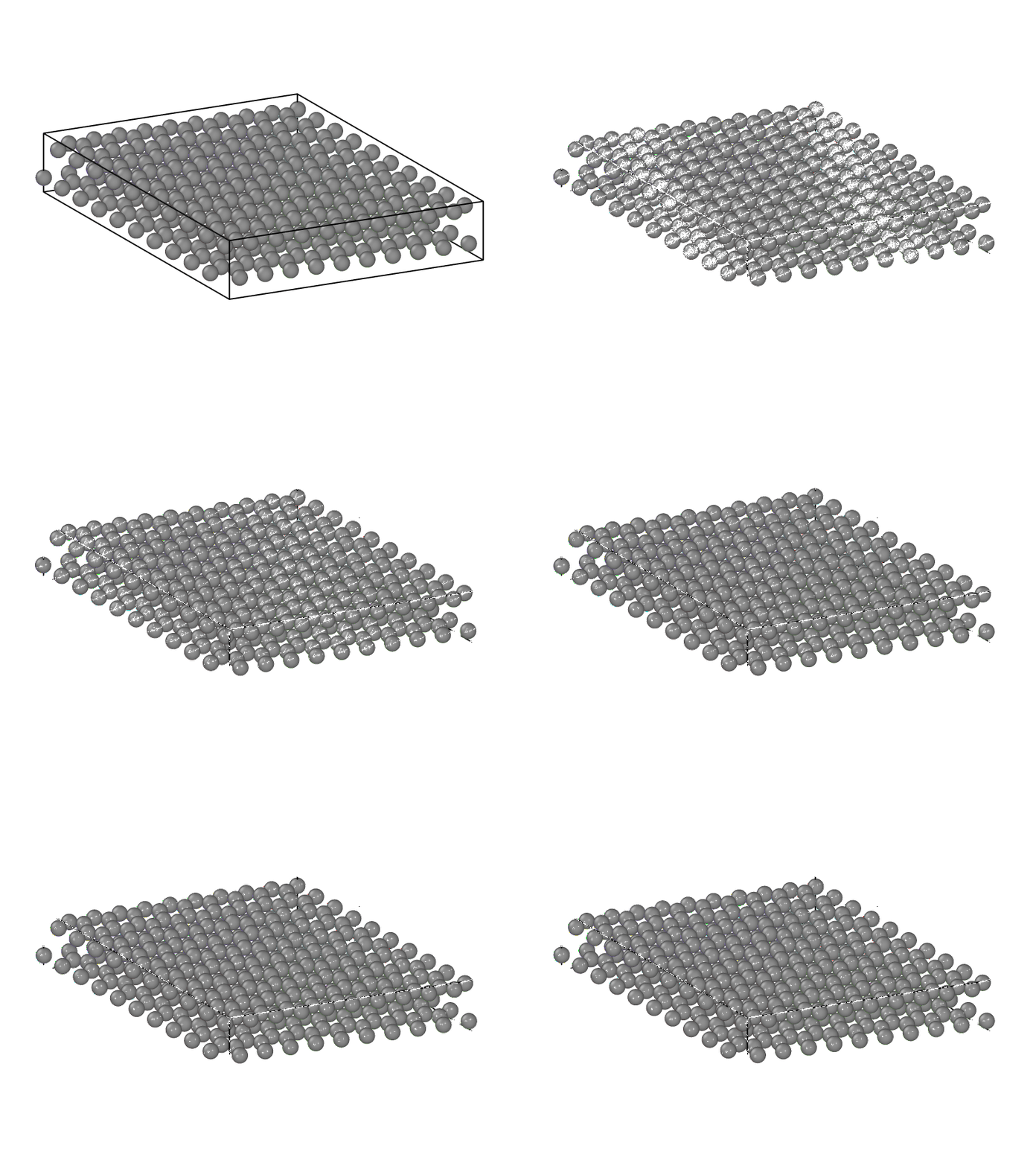
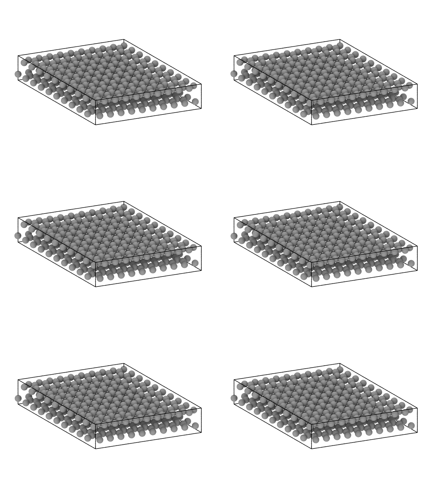
OVITO provides different renderers, and git output timing benchmark:
OpenGLRenderer: 0.78 s
TachyonRenderer: 16.09 s
OSPRayRenderer: 53.30 s
Also OpenGL is the fastest, the output quality is ill. Maybe Tachyon is the best choice for rendering.
[21]:
from ovito.io import import_file
# from ovito.data import *
from ovito.vis import Viewport
from ovito.vis import OpenGLRenderer, TachyonRenderer, OSPRayRenderer

kpt_idx, band_idx = 10, 2
pipeline = import_file(
    f"{ph_viz_dpath}/GK_kpt_{kpt_idx}_band_{band_idx}.xyz",
    columns = ["Particle Type", "Position.X", "Position.Y", "Position.Z"],
)
pipeline.add_to_scene()
atoms_frame_0 = read(f"{ph_viz_dpath}/GK_kpt_{kpt_idx}_band_{band_idx}.xyz", index=0)
center = atoms_frame_0.positions.mean(axis=0)
camera_pos_from_center = numpy.array((1, -1, 1))
vp = Viewport(
    type=Viewport.Type.Ortho,
    camera_pos = tuple(center + camera_pos_from_center),
    camera_dir=tuple(-camera_pos_from_center),  # look backwards to the center
)
vp.zoom_all()
vp.render_anim(
    size=(800,600),
    filename=f"{ph_viz_dpath}/GK_kpt_{kpt_idx}_band_{band_idx}.tachyon.gif",
    background=(1,1,1),
    fps=16,
    renderer=TachyonRenderer(),
)
pipeline.remove_from_scene()  # must remove, or the next import will be added to the scene and there will be multiple geometries
For TA (transverse acoustic) mode rendered by OpenGL:
For TA (transverse acoustic) mode rendered by Tachyon:
To visualize phonons locally in ovito, we need to generate an xyz file with phonon displacements. We provide the following two implementations:
In this tutorial, you can find xyz files containing phonon displacements in
${PROJECT_ROOT}/fd_runs/sc_5/ph_GK_viz_sc.The output is more or less like the results by OVITO python script above.
Please check this python script for creating xyz files from phonopy hdf5 output for ovito visualization and jmol visualization.
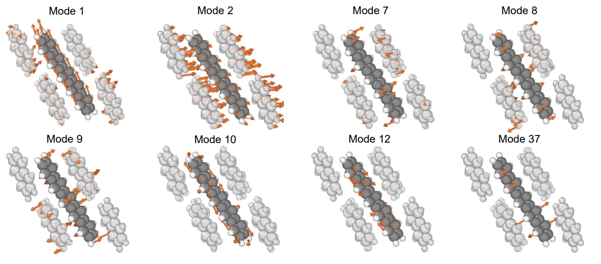
It visualizes phonon modes with arrows indicating displacement directions as below. Image from arXiV 2504.11224.