Momentum distributions from open path PIMD
Contributed by Hannah Bertschi
This tutorial shows how to set up an open path PIMD simulation in i-pi for the example of the water dimer. Furthermore, it describes how the output from i-pi can be used and processed to get the radial momentum distribution. Potential problems and how to test the results are provided as well.
Background
This section provides very minimal information on what equations are necessary to calculate the momentum distribution of an atom in a multi-atom molecule in three dimensions. For derivations please refer to [Pro]. The supporting information also contains important results.
The momentum distribution of atom \(k\) can be represented as a Fourier transform of the off-diagonal position matrix element of the density matrix \(e^{- \beta \hat{H}}/Z\)
The subscripts refer to the \(N\) atoms and \(\boldsymbol{q}\) is their three-dimensional position vector. The matrix element is off-diagonal, as there is a shift for atom \(k\) of \(\boldsymbol{\Delta}\). The position matrix element can be sampled by running path-integral molecular dynamics, where for atom \(k\) no spring connects the first and last bead.
In the end we want the radial momentum distribution, we know a priori that the momentum of an isolated molecule is isotropically distributed. After averaging over the angles we get
where \(\mathcal{N}_k(\Delta)\) can be sampled by running an open path PIMD simulation. The distance between the first and the last bead \(P\) of atom \(k\) given by \(|\boldsymbol{q}_k^{(P)} - \boldsymbol{q}_k^{(1)}|\) has to be calculated for each trajectory snapshot and then averaged via the following function
Here we use \(\sigma_P^2 = \hbar^2 \beta/P m_k\) with the inverse temperature \(\beta\), the number of beads \(P\) and the mass of the atom \(m_k\). Ultimately, \(\sigma_P\) is a convergence parameter, which we use to control the bandwidth of the Gaussian kernel that, effectively, is used to compute the end-to-end distance distribution by kernel density estimation.
i-pi inputs
Similar to standard PIMD we run a molecular dynamics simulation in the NVT ensemble with multiple beads. Most of the input keywords stay the same as compared to the standard PIMD. We will go here through an example xml input file and highlight what input is special for the open path simulations.
Some things to think about before/ when setting up the input file are (italic for what is shown in this example):
What is the temperature of interest? 60 K
How many beads are necessary for the chosen temperature and system? 64 beads
What potential to use? connection to MBX forcefield via unix socket
Is there already a PIMD simulation from which to restart? use RESTART-64 for initialization
For which atom do I want to calculate the momentum distribution, i.e. which atom(s) need an open path? one open path on atom 1 (hydrogen)
What thermostat and related parameters to use?
…
Note
The counting of indices in i-pi starts from zero. This is relevant for specifying the atom with an open path and its first and last beads.
Lets first look at what output to request:
<simulation verbosity='low'>
  <output prefix="simulation">
    <properties stride='40' filename='out'>
          [ step, time{picosecond}, conserved, temperature{kelvin}, kinetic_cv, potential, kinetic_cv(2), kinetic_cv(1) ]
    </properties>
    <properties stride='40' filename='H.q'> [ atom_x_path(1)] </properties>
    <trajectory bead='-16' format='xyz' filename='pos' stride='40'> positions </trajectory>
    <trajectory bead='63' format='xyz' filename='posn' stride='40'> positions </trajectory>
    <checkpoint filename="chk" stride="2000" overwrite="true"/>
  </output>
The momentum distribution depends on the distance between the first and last bead of the atom with the open path. Therefore these geometries need to be outputted. This is done in two ways here. The line <properties stride='40' filename='H.q'> [ atom_x_path(1)] </properties> outputs all the bead positions of atom 1 every 40 steps.
Other than writing all bead positions of the atom of interest, we can also write the geometries of all atoms of some specific beads. The line <trajectory bead='-16' format='xyz' filename='pos' stride='40'> positions </trajectory> outputs every 16nth bead of each atom, i.e. including bead 0. And the next line outputs the geometry of the last bead 63. Each bead is output in an XYZ file.
Either option gives us the geometries of atom 1 for the first and last bead. These we will need to process in the following section to get the momentum distributions.
Next in the xml file follows some generic information on the total steps and connection to a driver.
<total_steps>100000</total_steps>
  <prng>
    <seed>3348</seed>
  </prng>
  <ffsocket mode='unix' name='driver'>
    <address>mbx</address>
  </ffsocket>
Here we tell i-pi to use 64 beads and read a restart file, which corresponds to an equilibrated ring polymer structure, to initialize the simulation. The forces are just the ones returned by the driver.
<system>
  <initialize nbeads='64'>
    <file mode='chk'> RESTART-64 </file>
  </initialize>
  <forces>
    <force forcefield='driver'/>
  </forces>
This code block specifies the open path. In this case it is on atom 1, which is a hydrogen atom.
<normal_modes>
  <open_paths> [1] </open_paths>
</normal_modes>
Lastly follows all information on the NVT ensemble.
<ensemble>
  <temperature units='kelvin'>60.0</temperature>
</ensemble>
<motion mode='dynamics'>
  <dynamics mode='nvt' splitting='baoab'>
    <thermostat mode='pile_l'>
      <tau units='femtosecond'> 100 </tau>
    </thermostat>
    <timestep units='femtosecond'>0.25</timestep>
  </dynamics>
</motion>
</system>
</simulation>
The full input file can be downloaded here. The xyz files for the first and last <../_static/open_paths.pos_63.xyz> beads are also provided.
Processing the simulation output
The output geometries from the simulation are used to first calculate the distance between the first and last bead (in the code referenced as dist_H). Then the radial estimator in equation (2) has to be constructed. Below is some code showing how this can be done.
import numpy as np

def radial_estimator(delta, qP_q1, sigP):
    """
    Calculate the radial estimator for the end-to-end distance

    Args:
    delta (float one dimensional array): distances for which to
    evaluate the estimator, assumes 0 to be the first entry
    qP_q1 (float or one dimensional array): sampled distances
    of the last and first bead
    sigP (float): standard deviation of the Gaussians,
    sigP = sqrt(hbar^2 beta / (P m))

    Returns:
    N (one dimensional array): radial estimator as a
    function of delta (same length), is averaged over all qP_q1
    distances
    """
    D, q = np.meshgrid(np.asarray(delta[1:]), np.asarray(qP_q1))
    #delta in rows and qP_q1 in columns
    a = (2 * np.pi * sigP**2)**(-0.5) / (D * q)
    e1 = np.exp(-((D - q)**2)/(2 * sigP**2))
    e2 = np.exp(-((D + q)**2)/(2 * sigP**2))
    X = a * (e1 - e2)
    N = np.mean(X, axis=0) # average over qP_q1 values in columns
    # value at delta = 0
    N0 = 2 * (2 * np.pi)**(-0.5) * sigP**(-3) * np.mean(np.exp(-np.asarray(qP_q1)**2/(2 * sigP**2)))
    N = np.insert(N, 0, N0)
    return N
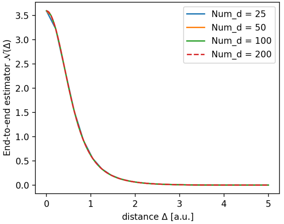
On a range of 0 to 5 for the delta variable I calculate the radial estimator for differing amounts of points Num_d.
Num_d = [25, 50, 100, 200]
ds = [np.linspace(0, 5, Nd) for Nd in Num_d]
N_s = [radial_estimator(delta=d, qP_q1=dist_H, sigP=sigH) for d in ds]
The resulting functions looks like this.
The radial momentum distribution is the given by the equation (1). A function that calculates this is:
def radial_momentum(delta, N, p, hbar=1):
    """
    Calculate the spherically averaged momentum distribution

    Args:
    delta (float or one dimensional array): distances for which
    the end-to-end distance is evaluated (first element is zero)
    N (one dimensional array): radial end-to-end estimator, same
    length as delta
    p (float or one dimensional array): momenta for which to calculate
    the distribution
    """
    P, D = np.meshgrid(np.asarray(p), np.asarray(delta))
    P, Nm = np.meshgrid(np.asarray(p), np.asarray(N))
    integrand = Nm[:,1:] * D[:,1:] * (hbar/P[:,1:]) * np.sin(P[:,1:] * D[:,1:] / hbar)
    integrand0 = np.asarray(N) * np.asarray(delta)**2 # evaluated at p=0
    integrand = np.hstack([integrand0.reshape(len(integrand0), 1), integrand])
    del_D = integral_del(D)
    av_int = integral_av(integrand)
    I = integrate(del_D, av_int)
    p_new = integral_av(p)
    n = 4 * np.pi * I
    return p_new, n
All code is provided in docs/source/open_paths/momentum_distribution.py file, also the integration fucntions used in the previous code.
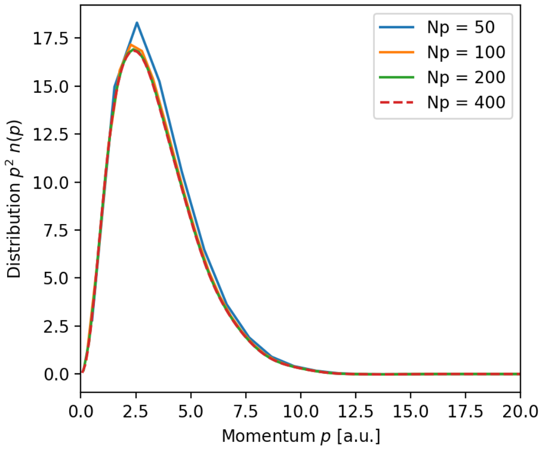
Trying different momentum grids and using the delta grid with 100 points
Num_p = [50, 100, 200, 400]
ps = [np.linspace(0, 50, N) for N in Num_p]
n_Hs = [radial_momentum(delta=ds[2], N=N_H, p=p) for p in ps]
gives plots like this
Note
The momentum distributions coming out of these formulas are not normalized. One has to normalize \(p^2 \ n(p)\) by its integral.
Things to keep in mind or make tests based on:
Test if the distributions are converged with respect to the simulation time
If there are multiple atoms of the same type (but different symmetry) check whether the open path is on each one equally is much
From \(p^2 \ n(p)\) you can calculate the kinetic energy, which can be compared to standard PIMD centroid-virial estimator
A harmonic analysis also allows calculation of the momentum distribution to compare to
References
Kapil, A. Cuzzocrea, and M. Ceriotti. Anisotropy of the Proton Momentum Distribution in Water J. Phys. Chem. B 122 6048-6054 (2018).